Design of a simple sphere deformer to displace a mesh model
Here are some thoughts about a very simple collision systems. The aim is to allow attaching spheres to a rig and repulse the skin around it.
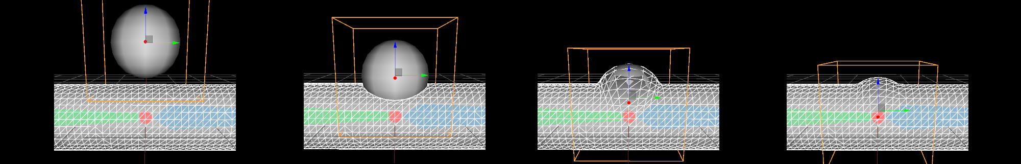
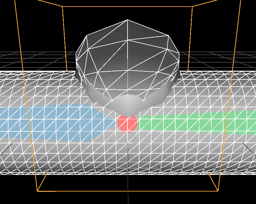
Let's start simple: we want to project the vertices of our mesh character on the surface of a sphere (c.f. introductory figure). Let \( \mathbf p \) be the vertex to deform and \( \mathbf c \) the center of our sphere of radius \(1\). When \( \mathbf p\) is inside the sphere (\( \| \mathbf p - \mathbf c \| < 1 \)) all you need is to normalize the vector going from \( \mathbf c \) to \( \mathbf p\) to obtain the needed displacement \( \mathbf disp = \frac{ \mathbf p - \mathbf c }{\| \mathbf p - \mathbf c \|} \).
Vec3 disp = (p - c);
float n = disp.norm();
if( n < 1.0f )
    out_vertex = c + (disp/n);
Now maybe a sphere is a bit too basic to use and we want to model ellipses. We want to enable the user to scale or rotate the sphere (in any direction). For this we attach a local frame to the center of the sphere. Therefore we define a \(4 \times 4\) transformation matrix \( T \) representing this local frame. We can express the displacement locally: before deforming the vertices we express them in the local frame \( \mathbf{p}_l = T^{-1} . \mathbf{p} \); the displacement becomes \( \mathbf{ disp }_l = \frac{ \mathbf{p}_l }{\| \mathbf{ p }_l \|} \) since the sphere's center in this coordinate system is now the origin. This displacement can be transformed back to global coordinates \( \mathbf{ disp } = T . \mathbf{ disp }_l \) to take into acount the various transformations.
Point3 lcl_vert = T.invert() * Point3(p); // p to the local coordinates of the sphere
Vec3 disp = lcl_vert;
float n = disp.norm();
if( n < 1.0f )
    out_vertex = c + (T * Vec3(disp/n)); // back to global coordinates and add displacement
 Non uniform scale along 'y' axis |
 scale and rotation |
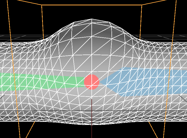
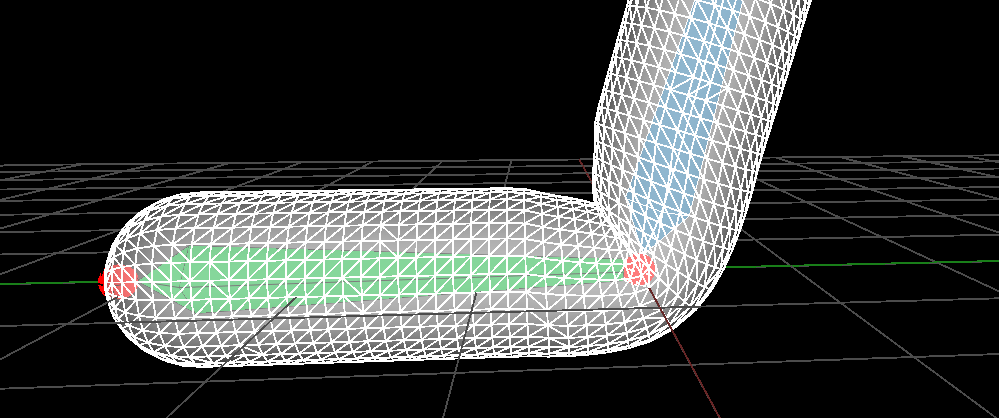
Ok, this is interesting but this deformation is not smooth at all: where the sphere's surface intersect our cylinder the transition is sharp. To get a smooth transition we need progessively push the vertices less and less outward the sphere. To do so we need to define a 'falloff function' mapping the distance from the center of the sphere to how much we push. Let's slightly re-write how we push the vertices:
float falloff(float);

Point3 lcl_vert = T.invert() * Point3(p);
Vec3 disp = lcl_vert;
float len = disp.norm();
out_vertex = p + (T * Vec3(disp * falloff(len)) );
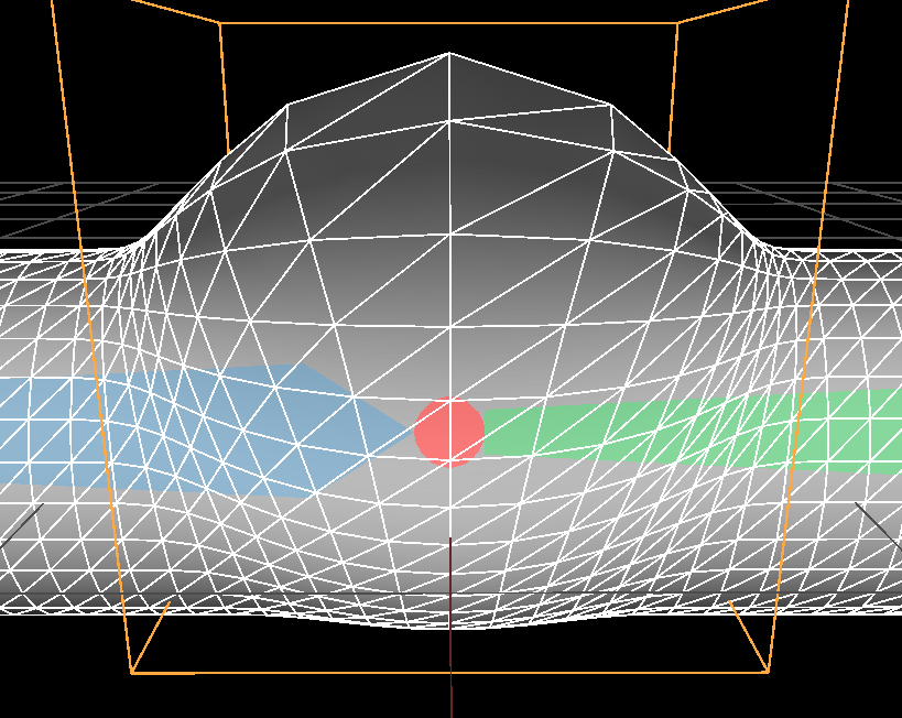
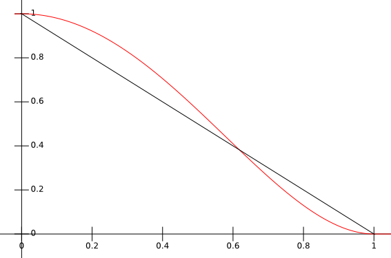
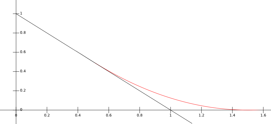
You should notice the transformed displacement is now added to the input vertex \(\mathbf p\) and not the center \(\mathbf c\) anymore. I could have kept \( \mathbf c \) but I think it's more intuitive to design the function falloff() as a function pushing the vertex \( \mathbf p \). Let's take a look at an example, if the function falloff looks like this:
 |
$$ falloff(x) |
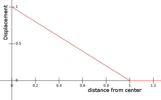
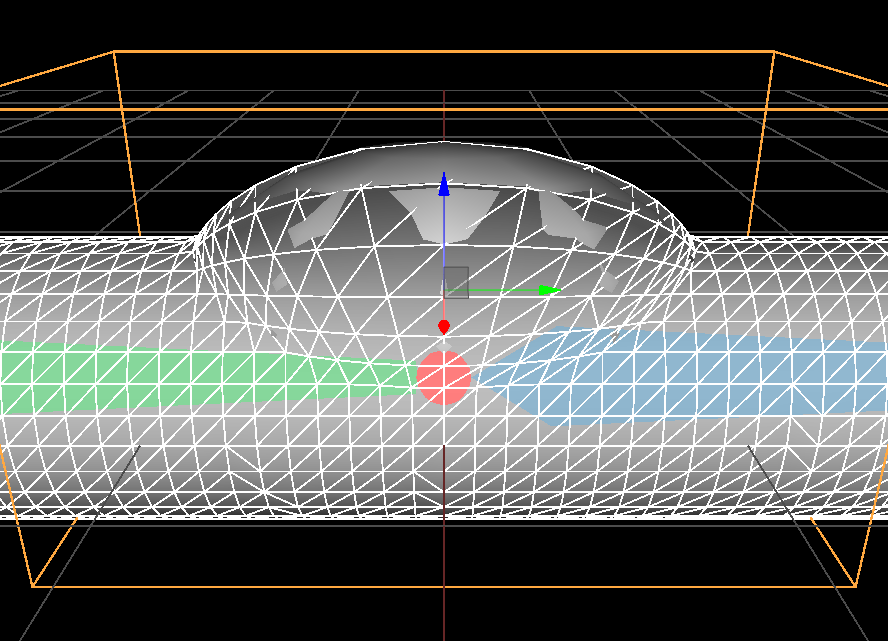
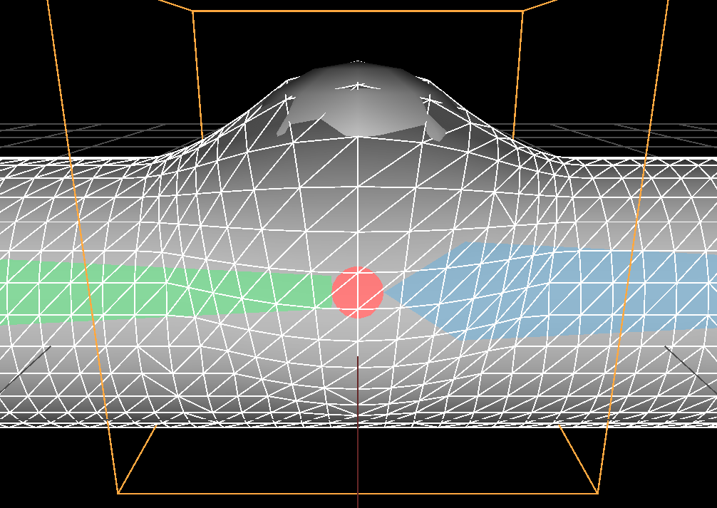
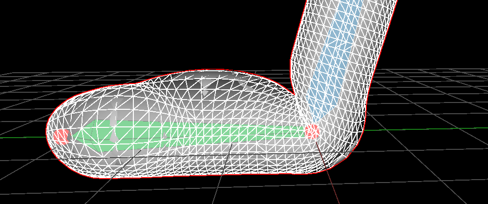
Then we obtain the results shown on the above figures where we perfectly fit the sphere surface. Notice how the function has a sharp angle at \( falloff(1) \) (the function is \(C^0\) ), this sharpness directly translates into a sharpness on the deformed mesh at the border of the sphere.
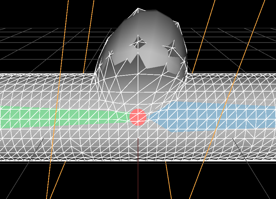
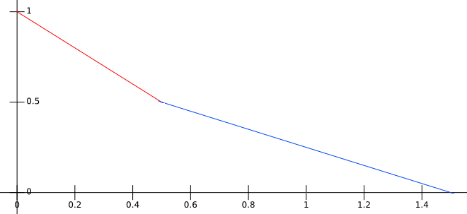
Here is another example of a piecewise linear falloff, I introduce a parameter \( 'r' \) allowing to influence beyond the sphere's radius:
 \( r = 1.5 \) |
$$ falloff_r(x) |
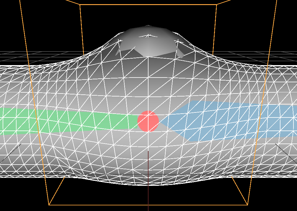 \( r = 2 \) |
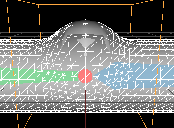
Possibilities are endless and we can explore a lot of different falloff functions. Here is a less pleasing (to me) deformation using the so-called blob function (a popular polynom used to model metaballs):
 \( r = 1 \) |
$$ falloff_r(x) |
 \( r = 2 \) |
One could let the user define the falloff function by using parametric curves (e.g. Bezier or Splines), but it would be slow to evaluate and impact the efficiency of the deformation algorithm. In our case I don't think we need this much freedom. Having just one parameter like the radius of influence should be enough and we can design a piecewise function fast to evaluate. Besides it will be simpler to use for the artist.
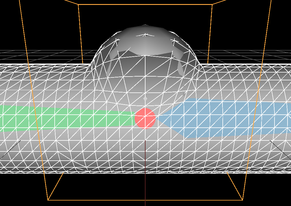
What I'm looking for is a deformation with vertices sticking as much as possible to the top of the sphere and then would get pushed a bit more than the radius of the sphere in a smooth fashion. So the piecewise linear function is almost good enough but we need to have smooth connections between the curves ( at least \( C^1 \)) so that the deformation look smooth. In addition I want a single parameter defining if we stick entirely to the sphere \( falloff(x) = (1-x) \) or if the transition has more influence and look smoother.
Given what we observed it means we want a curve closely following \( (1-x) \) around \( [ 0, 0.8] \) and then connect it to the abscissa with another curve above the line \( (1-x) \):
 \( r = 0.5 \) |
 $$ falloff_r(x) |
 \( r = 1 \) |
Here I simply connected a second degree polynom \(f =c_0 x^2 + c_1 x + c_2\) to the line \(1-x\) following these constraints:
$$ \left\{ \begin{array}{ll} f(r_1) = (1 - r_1) \\ f(r_2) = 0 \\ f'(r_1) = -1 \end{array} \right. $$If you solve this linear system of equations with your favorite Computer Algebra System (I personally love wxmaxima) you will find the above coefficients \(c_0, c_1\) and \( c_2 \).
/*Maxima commands to solve the system of equations: */
% f(x) := c_0*x^2+c_1*x+c_2;
% g(x) := diff(f(x), x);
% solve( [f(r_1) + r_1 = 1, f(r_2) = 0, g(r_1) =-1], [c_0,c_1,c_2] ), factor;
We now have a pretty simple falloff function with a single parameter \( r \) which defines how much we 'blend'. We can use several spheres if we add the displacement vectors, here are some more results with this solution:
 Standard linear blending |
|
 |
 |
| Three proxys and no blend (\( r = 0\)) | Three proxys with blendind (\( r = 0.5\)) |
Note 1: the constraints \( f(r_1) = (1 - r_1) \) and \( f'(r_1) = -1 \) are really important. It doesn't seem much but it took me a while to see I would get better results if the curve began with a \(1- x \) shape.
At first I was just trying solution with \( f(r_1) = 1 \) and it wasn't satisfying.
Note 2: in practice we prevent the user to set \(r = 0\) to avoid flickering of the lighting as well as the deformation (this happens at the intersection of the mesh and the sphere). It can be a good idea to impose a minimal radius such as \( r > 0.1 \).
Note 3: the computation of the displacement can be optimized when we use several objects by factorizing some of the matrix computations:
float falloff(float);

for(int j = 0; j < nb_proxys; ++j) {
    Mat44 T_inv = T[j].invert();
    for(int i = 0; i < nb_vertices; ++i) {
        Point3 p = vertex[i];
        Vec3 lcl_vert = T_inv * Point3(p);
        float len = lcl_vert.norm();
        // We simplified the matrix multiplication below
        // I recommend to not factorize 'len' division in 'falloff()'
        vertex[i] = vertex[i] + ((p - c) / len) * falloff(len);
    }
}
Normals
As explained in this other entry transforming the normal is done by computing the inverse transpose of the Jacobian of the deformation map i.e:
\[ \mathbf{n}_{out} = ( J\phi(x,y,z) )^{-T} . \mathbf{n}_{in} \]
In our case the deformation map is:
\[ \phi(\mathbf p) = \mathbf p + (\mathbf p - \mathbf c) . f( \| m(\mathbf p) \| ) \]
- With \( \mathbf c \) center of the sphere
- \( \phi: \mathbb R^3 \rightarrow \mathbb R^3 \) deformation map
- \( f: \mathbb R \rightarrow \mathbb R \) defined as \( f(x) = falloff(x) / x \)
- \( m: \mathbb R^3 \rightarrow \mathbb R^3 \) defined as \( m(\mathbf p) = T^{-1}.\mathbf p = M^{-1}.\mathbf p - \mathbf c \) it maps global coordinates to local coordinates of the sphere
- \( T \) the sphere frame represented as a \(4\times4\) matrix.
- \( M \) rotation of \( T \) i.e \(3\times3\) upper left matrix.
- \( \| \|: \mathbb R^3 \rightarrow \mathbb R \) vector length
Let's denote the jacobian as \(J \phi : \mathbb R^3 \rightarrow \mathbb R^{3\times3} \)
\[ J \phi =
\begin{bmatrix}
\nabla( \phi_x )^T \\
\nabla( \phi_y )^T \\
\nabla( \phi_z )^T
\end{bmatrix} =
\begin{bmatrix}
\dfrac{\partial \phi_x}{\partial x} & \dfrac{\partial \phi_x}{\partial y} & \dfrac{\partial \phi_x}{\partial z} \\
\dfrac{\partial \phi_y}{\partial x} & \dfrac{\partial \phi_y}{\partial y} & \dfrac{\partial \phi_y}{\partial z}\\
\dfrac{\partial \phi_z}{\partial x} & \dfrac{\partial \phi_z}{\partial y} & \dfrac{\partial \phi_z}{\partial z}
\end{bmatrix}
\]
Let's compute the Jacobian only on the \( x \) component of \( \phi_x:\mathbb R^3 \rightarrow \mathbb R\) which is the transposed gradient:
\[
\begin{align*}
\nabla \phi_x(\mathbf p)^T &= \nabla \left [ p_x + (p_x - c_x) . f( \| m(\mathbf p) \| ) \right ]^T \\
&= \nabla p_x + \nabla ( p_x - c_x) . f( \| m(\mathbf p) \| ) + (p_x - c_x) . \nabla \left [ f( \| m(\mathbf p) \| ) \right ]^T \\
&= (1, 0, 0) + (1, 0, 0) . f( \| m(\mathbf p) \| ) + (p_x - c_x) . \nabla \left [ f( \| m(\mathbf p) \| ) \right ]^T
\end{align*}
\]
Therefore if we expand the two other dimensions the Jacobian is:
\[
\begin{align*}
J \phi(\mathbf p) &=
\begin{bmatrix}
1 & 0 & 0 \\
0 & 1 & 0 \\
0 & 0 & 1
\end{bmatrix}
+
\begin{bmatrix}
1 & 0 & 0 \\
0 & 1 & 0 \\
0 & 0 & 1
\end{bmatrix}
. f( \| m(\mathbf p) \| ) +
\begin{bmatrix}
(p_x - c_x) . \nabla \left [ f( \| m(\mathbf p) \| ) \right ]^T \\
(p_y - c_y) . \nabla \left [ f( \| m(\mathbf p) \| ) \right ]^T \\
(p_z - c_z) . \nabla \left [ f( \| m(\mathbf p) \| ) \right ]^T
\end{bmatrix}
\end{align*}
\]
For the gradient we need to apply the chain rule twice:
\[
\begin{align*}
\nabla \left [ f( \| m(\mathbf p) \| ) \right ]^T &= f'( \| m(\mathbf p) \| ) . \nabla \left [ \| m(\mathbf p) \| \right ]^T \\
&= f'( \| m(\mathbf p) \| ) . \left ( J(m(\mathbf p))^T . \nabla \| m(\mathbf p) \| \right)^T \\
&= f'( \| m(\mathbf p) \| ) . \left ( (M^{-1})^T . \frac{m(\mathbf p)}{ \| m(\mathbf p) \| } \right)^T \\
&= f'( \| T^{-1} . \mathbf p \| ) . \left ( (M^{-1})^T . \frac{ T^{-1} . \mathbf p}{ \| T^{-1} . \mathbf p \| } \right)^T
\end{align*}
\]
Edge case
The jacobian is not always defined or invertible. In our case the Jacobian is ill defined for \( x < 1 - r \) of the falloff function which is when vertices verifies \( \| T^{-1} . \mathbf p \| < 1 - r \).
When this condition is met, vertices are projected onto the sphere no matter what their distance to the center \( \mathbf c \). Said differently, the vertices collides against the sphere surface when \( \| T^{-1}. \mathbf p \| < 1 - r \). Here is the problem: the Jacobian measure the variations of the deformation map, but when a vertex is colliding against an object there is no variations! Regardless of the vertex penetration into the collider it will always produce the same position (i.e on the surface of the collider). \( \phi \) is constant along the axis which projects the point onto the collider's surface therefore the variation is null.
In this case we shall not use the Jacobian.
Conclusion
Some results in video:
The final algorithm looks like this in pseudo C++ code:
float rad = /*some radius*/;

// falloff(x)
// defined for (x >= (1.0f - rad) && x < (1.0f + rad))
float falloff(float len)
{
    float x = len;

    float r1 = 1.0f - rad;
    float r2 = 1.0f + rad;
    assert( x >= r1 && x < r2);

    float r12 = r1 * r1;
    float r22 = r2 * r2;
    float denom = r22 - 2.0f * r1 * r2 + r12;
    float c0 = (r2 - 1.0f) / denom;
    float c1 = -(r22 + r12 - 2.0f * r1) / denom;
    float c2 = (r22 + r12 * r2 - 2.0f * r1 * r2) / denom;

    float res = c0 * x*x + c1 * x + c2;
    return res;
}

// f'(x) = df(falloff(x) / x) / dx' (i.e. first derivative)
// defined for (x >= (1.0f - rad) && x < (1.0f + rad))
float df(float len)
{

    float x = len;
    float r1 = 1.0f - rad;
    float r2 = 1.0f + rad;
    assert( x >= r1 && x < r2);

    float r12 = r1 * r1;
    float r22 = r2 * r2;
    float denom = r22 - 2.0f * r1 * r2 + r12;
    float c0 = (r2 - 1.0f) / denom;
    float c1 = -(r22 + r12 - 2.0f * r1) / denom;
    float c2 = (r22 + r12 * r2 - 2.0f * r1 * r2)/denom;

    float x2 = x*x;
    float res = ((2.0f * c0 * x + c1) / x) - ((c1 * x + c2 + c0 * x2) / x2);
    return res;
}

for(int j = 0; j < nb_proxys; ++j) {
    Mat44 T_inv = T[j].invert();
    for(int i = 0; i < nb_vertices; ++i) {
        Point3 p = vertex[i];
        Vec3 local_vert = T_inv * Point3(p);
        float len = local_vert.norm();
        // We only deform the vertices inside the radius of influence
        // of the sphere
        if( len < (rad + 1.0f) )
        {
            // Deform the vertex:
            Vec3 diff = p - c;
            if( len >= (1.0f - rad))
            {
                // Deform vertex
                float falloff_val = falloff(len);
                new_vertex = in_vertex + (diff/len) * falloff_val;

                // Transform normal with the inverse transpose of the Jacobian
                float falloff_scaled_prime = df(len);

                Vec3 grad = T_inv.get_mat3().transpose() * Vec3(local_vert / len);
                grad = grad * falloff_scaled_prime;

                Vec3 g0( (grad * diff.x) );
                Vec3 g1( (grad * diff.y) );
                Vec3 g2( (grad * diff.z) );

                Mat3 J(g0.x, g0.y, g0.z,
                       g1.x, g1.y, g1.z,
                       g2.x, g2.y, g2.z);

                J = Mat3::identity() + Mat3::identity() * (falloff_val / len) + J;

                J = J.inverse().transpose();
                new_normal = (J * Vec3(in_normal.normalized()));
           }
           else
           {
               // Deform vertex
               new_vertex = in_vertex + (diff/len) * (1.0f - len);

               // Jacobian is ill defined when we collide with the sphere.
               // So we compute normal directly by copying the normal
               // of the scaled sphere.
               Vec3 local_normal        = (T_inv * in_normal).normalized();
               Vec3 local_normal_sphere = Vec3(local_vert / len);
               float sign = local_normal.dot( local_normal_sphere ) < 0.0f ? -1.f : 1.f;
               new_normal = (T_inv.transpose() * local_normal_sphere) * sign;
           }
           new_normal.normalize();
       }
    }
}
 Donate
No comments