Normal to an implicit surface
Formal definition
The normal \( \overrightarrow n \) at a position \( \vec p(x,y,z) \in \mathbb R^3\) of a distance field \( f:\mathbb R^3 \rightarrow \mathbb R\) is computed with the gradient \( \nabla f \in \mathbb R^3 \):
$$ \overrightarrow{ n }( \vec p) = \frac{ \nabla f(x, y, z) }{ \| \nabla f(x, y, z) \| } $$The gradient is a vector of the partial derivatives of \( f \) in \( x\), \( y\) and \( z\):
$$ \nabla f(x,y,z) = \left[ \frac{\partial f(x,y,z)}{\partial x} , \frac{\partial f(x,y,z)}{\partial y} , \frac{\partial f(x,y,z)}{\partial z} \right] = \left[ f_x(x,y,z), f_y(x,y,z), f_z(x,y,z) \right] $$Note that sometimes implicit surface are represented with a compactly supported distance field, in this case the distance field \( f \) usually has decreasing values from the center of the primitive. Therefore, the gradient will point towards the opposite direction of the normal: \( \overrightarrow n = - \nabla f / \| \nabla f \| \)
Concrete application
If the above does not make any sense to you, here is a concrete example. Say you want to compute the normal vector of a sphere of centre \( \vec c \in \mathbb R^3\) and radius \( r \):
$$ \begin{array}{lll} f(\vec p(x,y,z)) & = & \| \vec p - \vec c \|^2 - r^2 \\ & = & ((x - c_x)^2 + (y - c_y)^2 + (z - c_z)^2) - r^2 \end{array} $$Then you need to compute \( \nabla f = (f_x, f_y, f_z) \):
$$ \begin{array}{lll} f_x(x,y,z) & = & (2).(1).(x-c_x)^{(2-1)} + 0 + 0 - 0 = 2(x-c_x)\\ f_y(x,y,z) & = & 2(y-c_y) \\ f_z(x,y,z) & = & 2(z-c_z) \end{array} $$In code:
float sphere(vec3 p, vec3 center, float radius){
    return squared_length( p - center ) - radius*radius;
}
vec3 sphere_gradient(vec3 p, vec3 center){
    return vec3( 2.0*(p.x - center.x), 2.0*(p.y - center.y), 2.0*(p.z - center.z));
}
vec3 sphere_normal(vec3 p, vec3 c){
    return normalize(sphere_gradient(p, c));
}
Finite difference
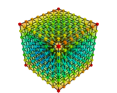
Say your function \( f \) is not defined with a mathematical formula,
instead, the values \(f(\vec p_1)\), \(f(\vec p_2)\), \( \cdots \), \(f(\vec p_n)\) are stored in a 3D texture.
Or perhaps you are feeling lazy and don't want to differentiate the analytical expression of \( f \).
There is still a way to find out \( \nabla f = (f_x, f_y, f_z) \) without knowing what's inside \( f \).
To this end, you can use what we call finite differences.
Recall how you differentiate a 1D function \( g: \mathbb R \rightarrow \mathbb R\) according to \( x \)
with the so called first order central difference:
Because our function \( f \) is multivariate (i.e. has several variables) the finite difference in \( x\), \( y\) and \( z\) are:
$$ f_x(x,y,z) = \frac{f(x+h,y,z) - f(x-h,y,z) }{2h} $$ $$ f_y(x,y,z) = \frac{f(x,y+h,z) - f(x,y-h,z) }{2h} $$ $$ f_z(x,y,z) = \frac{f(x,y,z+h) - f(x,y,z-h) }{2h} $$
Where \(h\) is usually a small number (e.g. 0.00001). This is called numerical differentiation, it is an approximation of the true value of \(f_x\), and usually, takes more time to compute than the analytical formula, however, it enables you to differentiate any function.
In code:
// For simplicity inlining center and radius
float sphere(vec3 p){
    vec3 center(0.0, 1.0, 0.0);
    float radius = 20.0;
    return squared_length( p - center ) - radius*radius;
}
vec3 sphere_gradient(vec3 p, vec3 c, float r){
    float h = 0.00001;
    // Note that the function sphere() can actually be replaced by any
    // function representing a distance field, since this approximation is universal
    float fx = (sphere(vec3(p.x+h, p.y, p.z)) - sphere(vec3(p.x-h, p.y, p.z))) / (2.0*h);
    float fy = (sphere(vec3(p.x, p.y+h, p.z)) - sphere(vec3(p.x, p.y-h, p.z))) / (2.0*h);
    float fz = (sphere(vec3(p.x, p.y, p.z+h)) - sphere(vec3(p.x, p.y, p.z-h))) / (2.0*h);
    return vec3( fx, fy, fz);
}
vec3 sphere_normal(vec3 p){
    return normalize(sphere_gradient(p));
}
Note:
Obviously for a sphere the only sane way to compute the normal is
\( \overrightarrow{ n }( \vec p) = normalized( \vec p - \vec{center}) \). But that's besides the point,
here we demonstrate how to generally compute a normal and gradient for any distance field.
Comparing your finite difference results with the analytical formula is a good way to check your computations though.
Optimized finite difference
In the above paragraph we need to evaluate the function of the distance field sphere() 6 times to compute the normal.
If this distance field does not actually represent a sphere, but rather a combination of thousands of complex objects, then each call to sphere() or similar, will be quite expensive.
There is another way to compute the normal with only 4 evaluations of \( f \). This is done using another finite difference scheme, the scheme is used as follows:
With \( \vec k_i \in \mathbb R^3 \) defined as the four following points in space:
$$ \vec k_i = \left \{ \vec k_1 = (1,-1,-1), \vec k_2 = (-1,-1,1), \vec k_3 = (-1,1,-1), \vec k_4 = (1,1,1) \right \} $$If you trust this formula then it translates to the following optimized code:
vec3 sphere_normal(vec3 p){
    float e = 0.00001;
    // Again sphere() can be any distance field function or combination of distance fields.
    return normalize( Vec3( 1, -1, -1) * sphere( p + Vec3( e, -e, -e) ) +
                      Vec3(-1, -1,  1) * sphere( p + Vec3(-e, -e,  e) ) +
                      Vec3(-1,  1, -1) * sphere( p + Vec3(-e,  e, -e) ) +
                      Vec3( 1,  1,  1) * sphere( p + Vec3( e,  e,  e) ) );
}
Origin of the 4 point finite difference
Although you can use this formula as is, for curious people, I leave below how this can be inferred. I was taught this trick by Íñigo Quílez. He kindly explained to me the mathematical reasoning behind it, which I'm transcribing here.
Here we use directional derivatives. Similarly to partial differentiation where we differentiate along one axis (\(x\), \(y\), \(z\), etc) we can differentiate along a specific unit vector \( \vec v \). In addition, directional derivatives can be expressed as a finite difference. The definition of the directional derivative \( \nabla_{\vec v}{f} : \mathbb R^n \rightarrow \mathbb R \) according to \( \vec v \) is as follows:
$$ \begin{array}{lll} \nabla_{\vec v}{f}(\vec p) & = & \nabla f(\vec p ) \cdot \vec v \phantom{---}\small{\text{ (dot product between the gradient and the direction)}}\\ & = & \lim_{h \rightarrow 0}{ (f(\vec p + h\vec v ) - f(\vec p)) / {h} } \end{array} $$
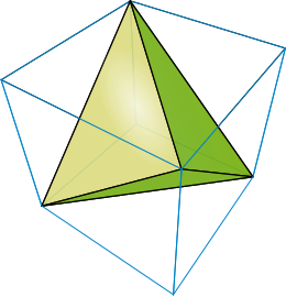
The trick consists in doing a weighted sum of four directional derivatives of \(f\):
$$ \begin{array}{lll} \overrightarrow{ m } & = & \sum\limits_i^{n=4} \vec k_i \nabla_{\vec k_i}{f}(\vec p) \\ & = & 4 \nabla f(\vec p) \end{array} $$Because we carefully chose four directions \( k_i \) pointing towards the four vertices of a regular tetrahedron, terms of this formula cancel out and simplify to the gradient of \( f \) !
First, let's see how the formula is related to finite difference:
$$ \begin{array}{lll} \overrightarrow{ m } & = & \sum\limits_i^{n=4} \vec k_i \nabla_{\vec k_i}{f}(\vec p) \\ & = & \sum\limits_i^{n=4} \frac{\vec k_i (f(\vec p + h\vec k_i ) - f(\vec p))}{h} \\ & = & \frac{\vec k_1 (f(\vec p + h\vec k_1 ) - f(\vec p))}{h} + \frac{\vec k_2 (f(\vec p + h\vec k_2 ) - f(\vec p))}{h} + \frac{\vec k_3 (f(\vec p + h\vec k_3 ) - f(\vec p))}{h} + \frac{\vec k_4 (f(\vec p + h\vec k_4 ) - f(\vec p))}{h} \\ & \phantom{=} & \\ & \phantom{=} & \text{Let's expand each component:} \\ m_x & = & \frac{\vec k_{1x} (f(\vec p + h\vec k_1 ) - f(\vec p))}{h} + \frac{\vec k_{2x} (f(\vec p + h\vec k_2 ) - f(\vec p))}{h} + \frac{\vec k_{3x} (f(\vec p + h\vec k_3 ) - f(\vec p))}{h} + \frac{\vec k_{4x} (f(\vec p + h\vec k_4 ) - f(\vec p))}{h} \\ m_y & = & \frac{\vec k_{1y} (f(\vec p + h\vec k_1 ) - f(\vec p))}{h} + \dots \\ m_z & = & \dots \end{array} $$It's a bit verbose so I'll try to find a more compact notation:
$$ \begin{array}{lll} \overrightarrow{ m } & = & \small \frac{1}{h} \left ( \begin{array}{r} k_{1x} (f(\vec p + h\vec k_1 ) - f(\vec p)) \\ k_{1y} (f(\vec p + h\vec k_1 ) - f(\vec p))\\ k_{1z} (f(\vec p + h\vec k_1 ) - f(\vec p)) \end{array} + \begin{array}{r} k_{2x} (f(\vec p + h\vec k_2 ) - f(\vec p) ) \\ k_{2y} (f(\vec p + h\vec k_2 ) - f(\vec p) ) \\ k_{2z} (f(\vec p + h\vec k_2 ) - f(\vec p) ) \end{array} + \begin{array}{r} k_{3x} (f(\vec p + h\vec k_3 ) - f(\vec p) )\\ k_{3y} (f(\vec p + h\vec k_3 ) - f(\vec p) )\\ k_{3z} (f(\vec p + h\vec k_3 ) - f(\vec p) ) \end{array} + \begin{array}{r} k_{4x} (f(\vec p + h\vec k_4 ) - f(\vec p)) \\ k_{4y} (f(\vec p + h\vec k_4 ) - f(\vec p)) \\ k_{4z} (f(\vec p + h\vec k_4 ) - f(\vec p)) \end{array} \right ) \begin{array}{r} \phantom{k_i}\\ \end{array} \\ \\ & = & \small \frac{1}{h} \left ( \begin{array}{r} k_1 \phantom{(f(\vec p + h\vec k_1 ) - f(\vec p))}\\ 1(f(\vec p + h\vec k_1 ) - f(\vec p)) \\ -1 (f(\vec p + h\vec k_1 ) - f(\vec p))\\ -1 (f(\vec p + h\vec k_1 ) - f(\vec p)) \end{array} + \begin{array}{r} k_2 \phantom{(f(\vec p + h\vec k_2 ) - f(\vec p))}\\ -1 (f(\vec p + h\vec k_2 ) - f(\vec p) ) \\ -1 (f(\vec p + h\vec k_2 ) - f(\vec p) ) \\ 1 (f(\vec p + h\vec k_2 ) - f(\vec p) ) \end{array} + \begin{array}{r} k_3\phantom{(f(\vec p + h\vec k_3 ) - f(\vec p))}\\ -1 (f(\vec p + h\vec k_3 ) - f(\vec p) )\\ 1 (f(\vec p + h\vec k_3 ) - f(\vec p) )\\ -1 (f(\vec p + h\vec k_3 ) - f(\vec p) ) \end{array} + \begin{array}{r} k_4\phantom{(f(\vec p + h\vec k_4 ) - f(\vec p))}\\ 1 (f(\vec p + h\vec k_4 ) - f(\vec p)) \\ 1 (f(\vec p + h\vec k_4 ) - f(\vec p)) \\ 1 (f(\vec p + h\vec k_4 ) - f(\vec p)) \end{array} \right ) \begin{array}{r} \phantom{k_i}\\ .[x]\\ .[y]\\ .[z] \end{array} \\ & \phantom{=} & \\ & = & \frac{1}{h} \left ( \begin{array}{r} f(\vec p + h\vec k_1 ) - f(\vec p) \\ -f(\vec p + h\vec k_1 ) + f(\vec p)\\ -f(\vec p + h\vec k_1 ) + f(\vec p) \end{array} \begin{array}{r} -f(\vec p + h\vec k_2 ) + f(\vec p) \\ -f(\vec p + h\vec k_2 ) + f(\vec p) \\ f(\vec p + h\vec k_2 ) - f(\vec p) \end{array} \begin{array}{r} -f(\vec p + h\vec k_3 ) + f(\vec p)\\ f(\vec p + h\vec k_3 ) - f(\vec p)\\ -f(\vec p + h\vec k_3 ) + f(\vec p) \end{array} \begin{array}{r} +f(\vec p + h\vec k_4 ) - f(\vec p) \\ +f(\vec p + h\vec k_4 ) - f(\vec p) \\ +f(\vec p + h\vec k_4 ) - f(\vec p) \end{array} \right )\\ & \phantom{=} & \\ & = & \frac{1}{h} \left ( \begin{array}{r} f(\vec p + h\vec k_1 ) \\ -f(\vec p + h\vec k_1 ) \\ -f(\vec p + h\vec k_1 ) \end{array} \begin{array}{r} -f(\vec p + h\vec k_2 ) \\ -f(\vec p + h\vec k_2 ) \\ f(\vec p + h\vec k_2 ) \end{array} \begin{array}{r} -f(\vec p + h\vec k_3 ) \\ f(\vec p + h\vec k_3 ) \\ -f(\vec p + h\vec k_3 ) \end{array} \begin{array}{r} +f(\vec p + h\vec k_4 ) \\ +f(\vec p + h\vec k_4 ) \\ +f(\vec p + h\vec k_4 ) \end{array} \right )\\ & \phantom{=} & \ \\ & = & \frac{1}{h} \left ( \vec k_1 f(\vec p + h\vec k_1 ) + \vec k_2 f(\vec p + h\vec k_2 ) + \vec k_3 f(\vec p + h\vec k_3 ) + \vec k_4 f(\vec p + h\vec k_4 ) \right )\\ & \phantom{=} & \ \\ & = & \sum\limits_i^{n=4} \vec k_i f(\vec p + h\vec k_i ) / h \\ \end{array} $$Nice, when using finite difference \( \overrightarrow{m} \) does simplify to only four evaluations of \( f\). Note that if you normalize you don't even need to divide by \( h \). Now how does \( \overrightarrow{m} \) relates to the gradient \( \nabla f \)?
$$ \begin{array}{lll} \overrightarrow{ m } & = & \sum\limits_i^{n=4} {\vec k_i \nabla_{\vec k_i}{f}(\vec p)} \\ & = & \sum\limits_i^{n=4}{ \vec k_i (\vec k_i \cdot \nabla f(\vec p)) } \text{ the operator }(\phantom{a}\cdot\phantom{a})\text{ represents the dot product} \\ & \phantom{=} & \\ & = & \sum\limits_i^{n=4} \begin{matrix} \vec k_{ix} \phantom{-}(\vec k_i \cdot \nabla f(\vec p)) \\ \vec k_{iy} \phantom{-}(\vec k_i \cdot \nabla f(\vec p)) \\ \vec k_{iz} \phantom{-}(\vec k_i \cdot \nabla f(\vec p)) \\ \end{matrix} \text{ exposing the components} \\ & \phantom{=} & \\ & = & \sum\limits_i^{n=4} \begin{matrix} (\vec k_{ix} \phantom{*} \vec k_i) \cdot \nabla f(\vec p) \\ (\vec k_{iy} \phantom{*} \vec k_i) \cdot \nabla f(\vec p) \\ (\vec k_{iz} \phantom{*} \vec k_i) \cdot \nabla f(\vec p) \\ \end{matrix} \text{ the dot product is associative with respect to scalar multiplication } \\ & \phantom{=} & \\ & = & \begin{matrix} \sum\limits_i^{n=4} (\vec k_{ix} \phantom{*} \vec k_i) \cdot \nabla f(\vec p) \\ \sum\limits_i^{n=4} (\vec k_{iy} \phantom{*} \vec k_i) \cdot \nabla f(\vec p) \\ \sum\limits_i^{n=4} (\vec k_{iz} \phantom{*} \vec k_i) \cdot \nabla f(\vec p) \\ \end{matrix} \\ & \phantom{=} & \\ & = & \begin{matrix} \nabla f(\vec p) \cdot \sum\limits_i^{n=4} (\vec k_{ix} \phantom{*} \vec k_i) \\ \nabla f(\vec p) \cdot \sum\limits_i^{n=4} (\vec k_{iy} \phantom{*} \vec k_i) \\ \nabla f(\vec p) \cdot \sum\limits_i^{n=4} (\vec k_{iz} \phantom{*} \vec k_i) \\ \end{matrix} \text{ the gradient is constant (does not depend on i) so we can take it out} \\ & \phantom{=} & \\ & \phantom{=} & \text{ Replace and compute with the coefficients of the vertices and let the magic happen:} \\ & \phantom{=} & \\ & = & \begin{matrix} \nabla f(\vec p) \cdot (4,0,0) \\ \nabla f(\vec p) \cdot (0,4,0) \\ \nabla f(\vec p) \cdot (0,0,4) \\ \end{matrix} \\ & \phantom{=} & \\ & = & 4 \nabla f(\vec p) \end{array} $$
And here you have it, the gradient scaled by a factor of 4.
Bonus
Matrix expression
In our previous development you can actually re-write the following as a matrix product of \(K \in \mathbb R^{3\times4} \):
$$ \begin{matrix} \nabla f(\vec p) \cdot \sum\limits_i^{n=4} (\vec k_{ix} \phantom{*} \vec k_i) \\ \nabla f(\vec p) \cdot \sum\limits_i^{n=4} (\vec k_{iy} \phantom{*} \vec k_i) \\ \nabla f(\vec p) \cdot \sum\limits_i^{n=4} (\vec k_{iz} \phantom{*} \vec k_i) \\ \end{matrix} \quad = \quad (K K^T) \ \ \nabla f(\vec p) $$Where:
$$ \begin{aligned} KK^T & = \begin{bmatrix} k_{1x} & k_{2x} & k_{3x} & k_{4x} \\ k_{1y} & k_{2y} & k_{3y} & k_{4y} \\ k_{1z} & k_{2z} & k_{3z} & k_{4z} \end{bmatrix} \begin{bmatrix} k_{1x} & k_{1y} & k_{1z} \\ k_{2x} & k_{2y} & k_{2z} \\ k_{3x} & k_{3y} & k_{3z} \\ k_{4x} & k_{4y} & k_{4z} \end{bmatrix} \\ & = \begin{bmatrix} \phantom{-}1 & -1 & -1 & \phantom{-}1 \\ -1 & -1 & \phantom{-} 1 & \phantom{-}1 \\ -1 & \phantom{-}1 & -1 & \phantom{-}1 \end{bmatrix} \begin{bmatrix} \phantom{-}1 & -1 & -1 \\ -1 & -1 & \phantom{-}1 \\ -1 & \phantom{-} 1 & -1 \\ \phantom{-}1 & \phantom{-} 1 & \phantom{-}1 \end{bmatrix}\\ & = \begin{bmatrix} 4 & 0 & 0 \\ 0 & 4 & 0 \\ 0 & 0 & 4 \end{bmatrix} \\ \\ & = 4I_3 \annotation{3 \times 3 \text{ identity matrix factor }4 } \end{aligned} $$Directional derivative for non-unit vector v
If \( \vec v \) is non-unit, the accurate formula of the directional derivative is:
$$ \begin{array}{lll} \nabla_{\vec v}{f}(\vec p) & = & \nabla f(\vec p ) \cdot \frac{\vec v}{\| \vec v\|} \\ & = & \lim_{h \rightarrow 0}{ \frac{(f(\vec p + h\vec v ) - f(\vec p)) }{ \| \vec v \|{h}} } \end{array} $$The tetrahedron's vertices presented here, define non unit vectors \( \|\vec k_i\| = \sqrt 3 \) from the origin. And we should actually have:
$$ \begin{array}{lll} \overrightarrow{ m } & = & \sum\limits_i^{n=4} \vec k_i \nabla_{\vec k_i}{f}(\vec p) \\ & = & \frac{4}{\sqrt 3 } \nabla f(\vec p) \end{array} $$But for the sake of clarity and not having to dangle on a scale factor everywhere in the formula, this was omitted. When the gradient is normalized to find the normal this doesn't change anything anyway.
Any scaling and rotation variant of the tetrahedron works
A very cool fact is that you can choose any set of points \(\vec k_i\) as long as they describe a regular tetrahedron centred at the origin. For instance:
{{ 0.942809041,-0.333333333, 0.0},
{-0.471404521,-0.333333333, 0.816496581},
{-0.471404521,-0.333333333,-0.816496581},
{ 0.0        , 1.0        , 0.0}};
Would work as well. You can try and plug the values to see you'll end up with the identity matrix up to scalar 'a' ( \(aI_3\) )
With standard linear algebra We can make prove that for any \(k_i\) of a regular tetrahedron the following holds:
$$ \begin{bmatrix} \sum\limits_i^{n=4} (\vec k_{ix} \phantom{*} \vec k_i) \\ \sum\limits_i^{n=4} (\vec k_{iy} \phantom{*} \vec k_i) \\ \sum\limits_i^{n=4} (\vec k_{iz} \phantom{*} \vec k_i) \\ \end{bmatrix} = KK^T = \begin{bmatrix} (a, 0, 0) \\ (0, a, 0) \\ (0, 0, a) \\ \end{bmatrix} = aI_3 $$First we show that for any rotation matrix \( R \):
$$ R^T aI_3 R = a(R^T I_3 R) = a (R^T R) = aI_3 $$Geometrically it should be obvious that rotating back and forth the unit basis vectors results in themselves. Algebraically the very definition of a rotation matrix is that it is and orthogonal matrix where \(R^T R = I \)
Now let's consider the rotated version of K that is \( K'= R^T K \), to complete our proof we'd like to show:
$$ K'{K'}^T = a I_3 $$Let's go:
$$ K'{K'}^T = R^T K (R^T K)^T = R^T K K^T R = R^T (K K^T) R = R^T aI_3 R = aI_3 $$And voila! Note that the same reasoning can be applied for scaling to fully generalize the proof.
Related
A while after writing this article Íñigo Quílez seems to have updated his article on numerical normals for SDF with the tetrahedron technique.
 Donate
No comments