Recipe for implicit surface reconstruction with HRBF

Compute distance field from point cloud data.

In this entry I'll explain and give code for the easiest method I know to reconstruct a surface represented by a scalar field \(f: \mathbb R^3 \rightarrow \mathbb R\) by interpolating a set of point with their normals. The method is called Hermite Radial Basis Function (HRBF) interpolation. The audience aimed is anyone with some basic knowledge about implicit surfaces (which people often know as metaballs and render with the marching cube algorithm)

Quick links:

• [  HRBF core sources ] [  HRBF toy app sources ] [  HRBF toy app binaries ] 
• [  maths details ]  [  maths summary ] [  tex sources (FR) (EN) ]

Method

An example

The goal is to build a surface \( f \) going through \( N \) points \( \mathbf p_i \), moreover the normals of \( f \) must match the user defined normals at each point \( \mathbf p_i \):

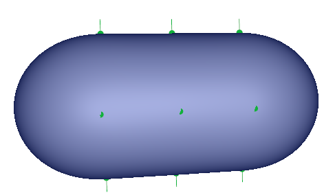
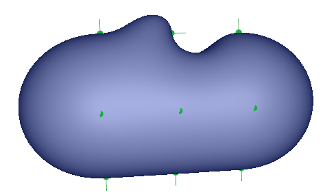
In these figures we can see two configurations. Here, points coordinates are the same, only a normal changes its direction (they are both represented in green). As we can see it plays an important role in the final shape of the surface. Using normals in addition to points has several advantages: the underlying algorithm will be more robust and easier to implement unlike other methods who only uses points (like standard RBF reconstruction). Also normals gives more control to the user like tangents used for 2D curves.

Other examples: look at the introductory figures, we see that when a point is too far away from the other points, a piece of surface gets separated from the main object producing a second piece of surface shaped like a bubble.

The maths

I'll split this section into two parts. First part (Conventions) I'll describe the conventions and basic notions I'm using, it's the easy part. The second part (Building the scalar field \( f \)) is more difficult but not mandatory to use the C++ code available below, however it will be useful to anyone who want to re-implement the method.

Conventions

So, given a set of \( N \) points and normals \( (\mathbf p_i, \mathbf n_i) \) we seek a scalar field \(f: \mathbb R^3 \rightarrow \mathbb R\). By convention we want \( f  \) to be equal to zero everywhere the surface lies. Since the surface must go through every points \( \mathbf p_i \) then \( f(\mathbf p_i) = 0\). Inside the shape \( f \) is negative and outside \( f \) is positive. The function \( f \) returns values ranging from \( [-\infty; +\infty ] \) and has increasing values from the inside to the outside. We say that \( f \) has a global support or is globally supported. It means the function varies everywhere in the ambient space \( \mathbf R^3 \).
It's worth noticing Metaballs are not defined with globally supported functions but compactly supported functions. Indeed the scalar field of a metaball decreases from the center until it vanishes to zero at the metaball's radius. So the function of a metaball stops varying outside its radius which means we can bound the variation inside a bounding box hence the name compactly supported. If you want to blend objects by summing them as you usually do with metaballs they have to be compactly supported. In this other entry I explain how to convert a globally supported scalar field to a compact support.

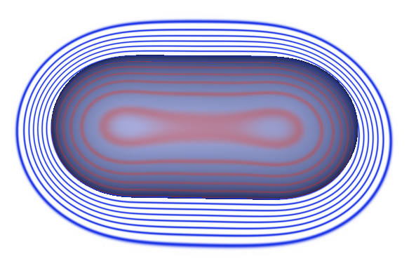
Here is a picture to help you visualize our function \( f \):

We see the surface for \(f(\mathbf p) \) = 0. Curves inside are red with \( f(\mathbf p) < 0\) and outside blue with \( f(\mathbf p) > 0\). What I did is cut the 3D space with a 2D plane and draw at regular interval curves. Every points that lies on the same curve  has the same scalar value of \( f \). For instance points at the frontier between blue and red are equal to zero. The next curve farther from the surface represent points for which \( f(\mathbf p) = 1 \) and so on. These curves are analog to contour lines in hiking maps but instead of representing the terrain elevation it tells the distance between a point and the implicit surface. (N.B: blue curves should continue indefinitely as the distance increases but I did not render all of them)

There is one thing I haven't defined yet which is how to compute the normals to the implicit surface. We have to compute what we call the gradient of the implicit surface which is written \( \nabla f \). The gradient return a vector which contains in each component the partial derivatives of \( f \):

$$ \nabla f = \begin{pmatrix}  \frac {\partial f(x, y, z)}{\partial x}, && \frac {\partial f(x, y, z)}{\partial y}, && \frac {\partial f(x, y, z)}{\partial z}
\end{pmatrix} $$

The gradient vector gives at any point of \( f \) the direction of steepest ascent i.e. the direction towards which \(f\) increases most. If you look back to the iso-curves you'll understand that the gradient is always orthogonal to the curves and hence to the implicit surface.  Indeed \( f \) doesn't vary if we follow a curve but increases the most when we go right through them.

Now we know how to compute the normal with \( \nabla f \) at any point of the implicit surface. In order to the implicit surface normals to match normals \( n_i \), we have to set \( \nabla f(\mathbf p_i) = \mathbf n_i \). This is what we have defined so far:

• At each point \( f(\mathbf p_i) = 0\) and \( \nabla f(\mathbf p_i) = \mathbf n_i \)
• Inside the object \( f(\mathbf p) < 0\)
• Outside the object \( f(\mathbf p) > 0\)

Building the scalar field \( f \)

Note: reading this section is not mandatory to use the C++ code.

Now comes the hard part: finding \( f \) that interpolates the set of points and normals \( (\mathbf p_i, \mathbf n_i) \). First we have to define what \( f \) looks like. How to find the form of \( f \) is outside the topic of this tutorial I'll just give the formula directly:

$$ f(\mathbf{x}) = \sum_i^N \mathbf{\alpha}_i \phi(\| \mathbf{x} - \mathbf{p}_i\|) +
\boldsymbol{\beta}_i . \nabla \left [\phi(\| \mathbf{x} - \mathbf{p}_i \|) \right ]$$

So with have \( \mathbf x \in \mathbb R^3 \) the evaluated position and \( \mathbf{p}_i \) the samples/points to be interpolated. The function \( \phi : \mathbb R \rightarrow \mathbb R \) is a called a radial basis function which I advice to define as \( \phi(x) = x^3 \). there are other possibilities but in my experience the method works best with \( x^3\). In order to be able to compute the value of \( f \) we will have to find the \( N \) values of \( \alpha_i \in \mathbb R \) and \( \boldsymbol{\beta}_i \in \mathbb R^3 \). Notice that \( \boldsymbol{\beta}_i \) and \( \nabla \phi \) being vectors \( \boldsymbol{\beta}_i . \nabla \phi \) is the dot product. In order to find the unknown \( \alpha_i \) and \( \boldsymbol{\beta}_i \) we have to solve this linear system of equations:

$$ \begin{pmatrix}
 f( \mathbf{p}_i ) \\
 \nabla f( \mathbf{p}_i )
\end{pmatrix}=
\begin{pmatrix}
  0 \\
  \mathbf{n}_i
\end{pmatrix} $$

As we said before points on the surface are associated to the value zero and normals and gradient must match. For this system I'm using a rather compact notation because there is actually \( 4N \) lines with \( 4N \) unknown. As it would take too much space I have put all the [  developments details in a pdf ]. If you're not interested in the developments I've made a [  summary with only the detailed matrix ] to solve the system.

Interpreting the formula of \( f \)

It may be a bit abstract to understand how summing the expression \( \mathbf{\alpha}_i \phi(\| \mathbf{x} - \mathbf{p}_i\|) +
\boldsymbol{\beta}_i . \nabla \left [\phi(\| \mathbf{x} - \mathbf{p}_i \|) \right ] \) with appropriate weights \( \mathbf{\alpha}_i \) and \( \boldsymbol{\beta}_i \) gives a correct interpolation of the implicit surface. Lets take an example and draw the implicit surface:

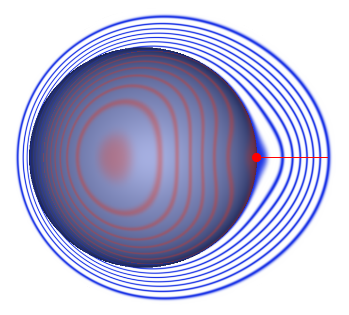
$$ g(\mathbf x) = 1 \phi(\| \mathbf{x} \|) + (1,0,0) . \nabla \left [\phi(\| \mathbf{x} \|) \right ]  $$

It's a single HRBF centered at \( (0, 0, 0) \) with \( \mathbf{\alpha}_i = 1 \) and \( \boldsymbol{\beta}_i = (1, 0, 0) \) which looks like this:

The point position in red is \( (0,0,0) \) and the normal direction is \( (1,0,0) \). So we can observe that each point correspond to a blob like function. However the blob is not centered at the point position but its surface goes through the point. Moreover the normal controls the orientation of this blob. So the intuition is that by blending all the blobs with a sum we generate a final object whose shape goes through all the points.

Code

The essential

The C++ code for HRBF interpolation uses the library Eigen to solve the linear system. Fortunately it's a header library. It means you won't have to compile/install it because it is only composed of headers. They are readily usable within any projects using the #include directive. The [  HRBF C++ code ] should not be hard to use. The class takes in input a vector of points and normals to compute the surface as shown here:

#include "hrbf_phi_funcs.h"
#include "hrbf_core.h"

typedef HRBF_fit<float, 3, Rbf_pow3<float> > HRBF;

{
    HRBF fit;
    // Define samples (position, normal);
    HRBF::Vector pts[] = { HRBF::Vector( 0.f, 0.f, 0.f), HRBF::Vector( 1.f, 0.f, 0.f), HRBF::Vector( 0.f, 0.f, 2.f) };
    HRBF::Vector nrs[] = { HRBF::Vector(-1.f, 0.f, 0.f), HRBF::Vector( 1.f, 0.f, 0.f), HRBF::Vector( 0.f, 0.f, 1.f) };

    const int size = sizeof(pts) / sizeof(HRBF::Vector);
    std::vector p(pts, pts + size );
    std::vector n(nrs, nrs + size );
    // Solve linear system;
    fit.hermite_fit(p, n);
}

Then the implicit surface potential can be easily evaluated at any point of the ambiant space:

HRBF::Vector x( 0.f, 0.f, 0.f);
float potential = fit.eval( x );
HRBF::Vector gf = fit.grad( x );

Note also that the code works for any dimensions, for instance in 2D you can easily generate the function of an implicit curve \( f: \mathbb R^2 \rightarrow \mathbb R \)

typedef HRBF_fit<float, 2, Rbf_pow3<float> > HRBF_curve;

Performances

Be aware compiling in Debug mode is a lot slower than Release mode to solve linear systems.

The toy application

In order to do some testing rapidly I provide a toy application. It enables the edition of HRBF points and the visualization with a marching cube algorithm. There is also an automatic bounding box fitting around the HRBF. Feel free to play and modify the program:

• [  HRBF toy app sources ]
• [  HRBF toy app binaries ] (linux x64 and windows x86)

Reference:

Hermite Interpolation of Implicit Surfaces with Radial Basis Functions; Ives Macêdo & Al

---

six comments

Name

Email (optional field, I won't disclose or spam but it's necessary to notify you if I respond to your comment)

All html tags except <b> and <i> will be removed from your comment. You can make links by just typing the url or mail-address.

Anti-spam question:
√4 + 40 = ?

There are more things in heaven and earth,
Horatio, than are dreamt of in your philosophy.
-- Wm. Shakespeare, "Hamlet"