Dual Quaternions skinning tutorial and C++ codes

日本語版・Japanese version

In this entry I provide [  C++ codes ] to deform a mesh with the famous Dual Quaternion Skinning (DQS) deformer.

This tutorial aims to present and explain the general idea behind Dual Quaternions and give means to integrate it quickly into a pre-existing Linear Blending Skinning (LBS) pipeline. My goal is to give the minimal set of explanations to re-use my code quickly. Therefore I will try not to dwell too much on the maths which are thoroughly explained in the original paper: "Geometric Skinning with Approximate Dual Quaternion Blending". I will also assume the reader have some basic knowledge about Skeletal Animation and Quaternions (used as a mean to represent 3D rotations).

LBS: the loss of volume issue

Lets briefly recall how Linear Blending Skinning is done and its main limitation. The aim is to deform a mesh model using a set of bones forming a skeleton:

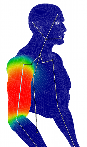
Manually or automatically each bone is associated to parts of the mesh. The figure shows the influence of one bone over the mesh. Red means the vertex is associated to a weight equal to 1 (it'll match exactly the bone motion). Green means mid-influence with a weight of 0.5. Finally blue means a weight of 0 (no motion related to this bone). Each bone defines a complete set of weights over the mesh. Moreover the bones influences usually overlap to produce a smooth transition between the joints. Here is the formula to compute the deformation of the mesh:

$$ \begin{equation}
\bar{\mathbf{p_i}} = \sum_{j=1}^{n} w_{ij}  T_j  \mathbf{p_i}
\end{equation} $$

Where \(n\) defines the number of bones, \(w_{ij}\) is a scalar weight at the i\(^{\text{th}}\) vertex associated to the j\(^{\text{th}}\) bone and \(T_j\) the 4x4 matrix which defines a global transformation of the j\(^{\text{th}}\) bone from its rest pose. Finally \(\mathbf{p_i}\) is a mesh's vertex in rest pose and \(\bar{\mathbf{p_i}}\) the vertex after deformation. Usually the weights \(w_{ij}\) are normalized at each vertex to sum to one \(\sum_{j=1}^{n} w_{ij} = 1\). The schematic below illustrates the problem of loss of volume when bending or twisting with LBS:

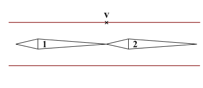
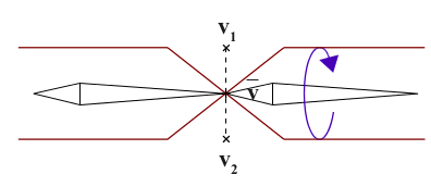
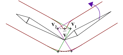
Here the central vertex \(\mathbf v\) is equally influenced by both bones therefore \(w_{i1} = w_{i2} = 0.5\). looking closer to the LBS equation in this simple example:

$$
\begin{eqnarray}
\bar{\mathbf{v}} &= & \sum_{j=1}^{n} w_j T_j \mathbf{v} \\
                             &= & w_1 (T_1 . \mathbf v) + w_2 (T_2 . \mathbf v) \\
                             &= & 0.5 \mathbf{v_1} + 0.5 \mathbf{v_2}
\end{eqnarray}
$$

We can see that the linear interpolation between \(\mathbf v_1\) and \(\mathbf v_2\) produces \(\bar{ \mathbf v}\) at a inadequate location which result in the loss of volume. Another way to understand why there is such contraction of the mesh is to look at the matrices:

$$
\begin{eqnarray}
\bar{\mathbf{v}} &= & \sum_{j=1}^{n} w_j T_j \mathbf{v} \\
                             &= & (w_1 . T_1  + w_2 . T_2) . \mathbf v \\
                             &= & M . \mathbf v
\end{eqnarray}
$$

Even if \(T_1\) and \(T_2\) are rigid transformations (i.e exclusively express rotation and translation) their weighted combination is not guaranteed to be a rigid transformation. As a matter of fact a scale factor often appear in \(M\) hence the shrinkage. More on computing \(T_j \) here.

Dual Quaternions Skinning

Introduction

Dual Quaternion Skinning (DQS) is a good alternative to Linear Blending Skinning (LBS) (sometime called Smooth Skinning or SSD for Skeletal Subspace Deformation) to avoid the loss of volume problem. DQS is almost as fast as LBS and as easy to implement (once you've understood the math of course). You can test DQS in a lot of software such as Maya, 3D Studio Max or Blender (see my entry on how to setup a cylinder to test DQS in Blender). 

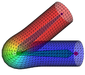
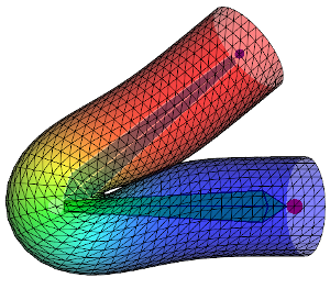
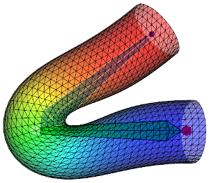
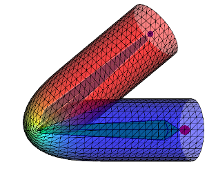
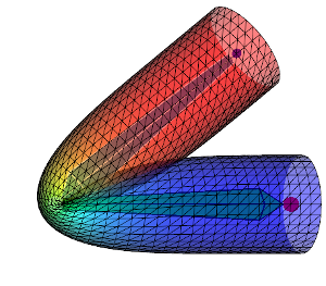
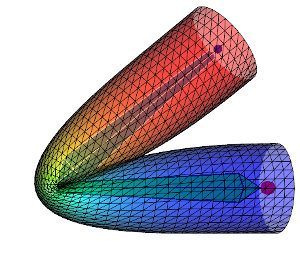
Here are some figures which compare DQS and LBS on a cylinder with different influence weights:

Dual Quats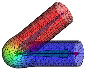
Linear  Blend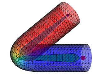
Weight diffusion	+	++	+++	++++

First row shows the DQS and second row the LBS. From left to right the influence weights are more and more diffused over the mesh therefore the deformation is smoother. Keep in mind that the aspect of the deformation can vary a lot depending on how the weights are diffused. When going away from a bone the weights \(w_{ij}\) can decrease more less rapidly (linearly, quadratically ...) and affect the look of the deformation. All this to say: to get the same results as above using my code you would need to get the exact same influence weights.

The idea

This is a informal explanation of why the problem of loss of volume can be corrected using Dual Quaternions Skinning. The idea can be summarized with the schematic below (reproduced from the original paper):

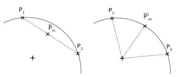
The left figure would be the LBS between two vertices. It is a linear interpolation and the new position will be somewhere lying on the segment between \(\mathbf{p_1}\) and \(\mathbf{p_2}\). On the right would be the DQS, instead of a linear interpolation it is a spherical one. The new position will be lying on the arc circle instead which will avoid the mesh' shrinkage.

So how is it performed? Instead of using matrices to express the motions of the joints DQS will use mathematical objects called Dual Quaternions. Note that it's easier to understand what Dual Quaternions are if you already used Quaternions (if not this tutorial should be enough for our purpose). So one day you may have learn to use complex numbers to express 2D rotations which you can also do with a 2x2 matrix. Then you may have seen the extension of complex: the Quaternions. With them you can express 3D rotations as you would do with a 3x3 matrix. Well now you can use Dual Quaternions which can express a rotation and a translation like a 4x4 matrix.

So this is how we compute the deformed position of a vertex with DQS:

$$ \mathbf{\dot q} =
\frac{\sum_{i=1}^n w_i \mathbf{\dot q}_i}{\| \sum_{i=1}^n w_i \mathbf{\dot q}_i \|}
$$

Instead of blending matrices (\( M = \sum_{i=1}^{n} w_i T_i \)) we blend Dual Quaternions. Here \(\mathbf{\dot q}_i\) is the bone's dual quat transformation weighted by \(w_i\). The result is normalized with \( {\| \sum_{i=1}^n w_i \mathbf{\dot q}_i \|} \) to produce the final Dual Quaternion used to transform a vertex from rest pose to the deformed position. Even if you don't know how to manipulate Dual Quaternions (i.e add/multiply/divide or transform points with them), I can give you the intuition of why it is better than LBS. The above blending of Dual Quaternions will compute a new Dual Quaternion which is guaranteed to represent only a rotation and a translation. This means unlike matrix blending there won't be any scale factor shrinking the mesh around joints.

The recipe

This is the things we need to know to implement DQS into a pre-existing LBS software:

1. How to represent dual quaternions (it's basically eight real numbers)
2. How to convert a 4x4 matrix to Dual Quaternions
3. How to compute the needed operators on Dual Quaternions such as: * + /
4. How to apply the transformation of a Dual Quaternion to a vertex

All these questions are answered by the authors in the original paper section 4 so I will try to be brief on the math.  Besides everything can be inferred/extracted from my [  code ].

1. Representation

First Dual Quaternions are Dual numbers. A Dual Number is a number of the form \(a + \varepsilon b\) where \( \varepsilon^2 = 0 \) (Sounds like the story of Complex Numbers...). Well if \(a\) and \(b\) are Quaternions we get a Dual Quaternion \(\mathbf{\dot q} = \mathbf q_0 + \varepsilon \mathbf q_e\). Which means we need eight floats to store it (four floats per Quaternions)

2. Conversion

Now we need to initialize correctly those value for the Dual Quaternion to represent the correct translation and rotation of the  bone. It can be done easily using the Dual Quaternion constructor:

#include "dual_quat_cu.hpp" 
using namespace Tbx;
{
    Transfo mat; // 4x4 matrix representing the transformation of a bone
    Dual_quat_cu dq( mat ); // Building dual quaternion from matrix
}

Which convert the rotation part of the matrix to a Quaternion and extract the vector of translation. The Quaternion and translation vector are then converted to a single Dual Quaternion as describe in the paper.

3. Operators

To perform the blending of Dual Quaternions you need to know how to compute things like the addition of Dual Quaternions or even multiplying by a scalar. Again all this is covered by the paper or can be inferred by looking at the overloaded operators in the Dual Quaternion class.

4. Apply transformation

I provide the method transform() and rotate() to transform a point or rotate a vector using the Dual Quaternion.

Deformer code

Here is an example to perform the Dual Quaternion Blending on a mesh. You will notice a suspicious "if" statement performing a sign test. This test is done to ensure the shortest rotation path is taken:

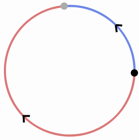
The dot product's sign between two Dual Quaternions will help determine the shortest path. This is explained section 4.1 of the paper.

#include <vector>
#include "dual_quat_cu.hpp"

using namespace Tbx;

/**
 * @param in_verts : vector of mesh vertices in rest positon 
 * (model coordinates)
 * @param in_normals : vector of mesh normals (same order as 'in_verts')
 * @param out_verts : deformed vertices with dual quaternions
 * @param out_normals : deformed normals with dual quaternions
 * @param dual_quat : list of dual quaternions transformations per joints
 * (each dual quat transforms vertices in model coordinates)
 * @param weights : list of influence weights for each vertex
 * @param joints_id : list of joints influence fore each vertex
 * (same order as 'weights')
 */
void dual_quat_deformer(const std::vector<Point3>& in_verts,
                        const std::vector<Vec3>& in_normals,
                        std::vector<Vec3>& out_verts,
                        std::vector<Vec3>& out_normals,
                        const std::vector<Dual_quat_cu>& dual_quat,
                        const std::vector< std::vector<float> >& weights,
                        const std::vector< std::vector<int> >& joints_id)
{
    for(unsigned v = 0; v < in_verts.size(); ++v)
    {
        // Number of joints influencing vertex 'v'
        const int nb_joints = weights[v].size(); 

        if(nb_joints != 0)
        {
            Dual_quat_cu dq_blend = Dual_quat(Quat(0.0f, 0.0f, 0.0f, 0.0f), 
                                              Quat(0.0f, 0.0f, 0.0f, 0.0f));

            int pivot = joints_id[v][0];
            Quat_cu q0 = dual_quat[pivot].rotation();
            // Look up the other joints influencing 'p' if any
            for(int j = 0; j < nb_joints; j++)
            {
                const int k = joints_id[v][j];
                float w = weights[v][j];
                const Dual_quat_cu& dq = (k == -1) ? Dual_quat_cu::identity() : dual_quat[k];
                // Seek shortest rotation:
                if( dq.rotation().dot( q0 ) < 0.f )
                    w *= -1.f;

                dq_blend = dq_blend + dq * w;
            }            
        }else{
            dq_blend = Dual_quat::identity();
        }

        // Compute animated position
        Vec3 vi = dq_blend.transform( in_verts[v] ).to_vec3();
        out_verts[v] = vi;
        // Compute animated normal
        out_normals[v] = dq_blend.rotate( in_normals[v] );
    }
}
 

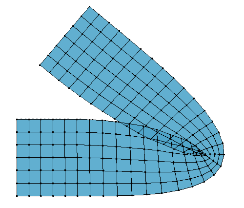
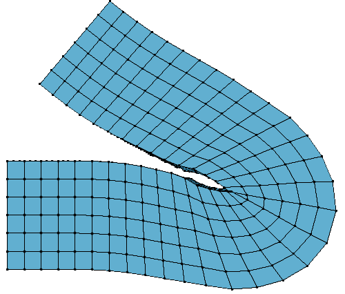
Another comparison between LBS (left) and DQS (right):

Conclusion

DQS has become the second standard after LBS in the industry. It is fast and easy to implement (especially if the codes for the Dual Quaternion mathematics are already provided).

You may have noticed in the above figures the tendency of DQS to produce a bulge around the joints. This is more or less visible given certain skinning weights. This problem was not discussed in the original paper but since then there has been a few developments. I provide codes to implement a quick fix of the Dual Quaternion Skinning bulge artifact. There is also a Disney paper providing a more elegant and robust solution Real-time Skeletal Skinning with Optimized Centers of Rotation. The later is a bit more tedious to implement though.

Discussed in the paper section 4.2 but not here, is how to handle scale and shear transformations with DQS, you can find more details in this other blog post.

Links:

Some additional resources:

C library for Dual-Quaternions
A more formal tutorial on Dual Quaternions Skinning
Maya plugin

Reference:

Geometric Skinning with Approximate Dual Quaternion, Ladislav Kavan & Al

three comments

Name

Email (optional field, I won't disclose or spam but it's necessary to notify you if I respond to your comment)

All html tags except <b> and <i> will be removed from your comment. You can make links by just typing the url or mail-address.

Anti-spam question:
√4 + 40 = ?

Innovation is disobedience.
(Fr: Innover c’est désobéir.)
-- Iddriss Aberkane? Pr Raoult? XD