Curvature of a Distance field / Implicit surface

Draft notes
Curvature signed distance field (SDF), implicit surface, level set.
Good reference list various curvature formula for implicit curves / surfaces (distance field):
"Goldman, R. (2005). "Curvature formulas for implicit curves and surfaces". Computer Aided Geometric Design. 22 (7): 632–658. doi:10.1016/j.cagd.2005.06.005"
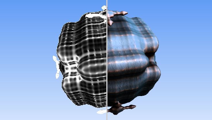
Mean Curvature
Mean curvature with cheap evaluation:
//Cheap curvature by nimitz (twitter: @stormoid)

/*
	Not sure if this method is new, but I haven't seen it around.
	Using a single extra tap to return analytic curvature of an SDF.

	My first implementation required 16 taps, then 12, then thanks
	to some math help from a friend (austere) I got it down to 7 taps.
	And this is the	final optimization which requires 5 taps or a
	single tap if you're already computing normals.


	Edit (April 2016):

	Coming back to this I know realize that what I am returning is an
	approximation of the Laplacian of the SDF and the Laplacian being
	the divergence of the gradient of the field means that any point
	on the surface being a sink will return negative "curvature" and
	vice-versa (since the gradient of a SDF should point to the centroid
	at any point in space).

	So now, I include the 7-tap version which is a more accurate Laplacian,
	while the 5-tap version while cheaper, it is less accurate.

	N.B. Mean curvature is computed here, not Gaussian curvature. (thanks to Fabrice)
*/

#define ITR 80
#define FAR 10.
#define time iTime

mat2 mm2(in float a){float c = cos(a), s = sin(a);return mat2(c,s,-s,c);}

float map(vec3 p)
{
    p.x += sin(p.y*4.+time+sin(p.z))*0.15;
    float d = length(p)-1.;
    float st = sin(time*0.42)*.5+0.5;
    const float frq = 10.;
    d += sin(p.x*frq + time*.3 + sin(p.z*frq+time*.5+sin(p.y*frq+time*.7)))*0.075*st;

    return d;
}

float march(in vec3 ro, in vec3 rd)
{
	float precis = 0.001;
    float h=precis*2.0;
    float d = 0.;
    for( int i=0; i<ITR; i++ )
    {
        if( abs( h ) < precis || d > FAR ) break;
        d += h;
	    float res = map(ro+rd*d);
        h = res;
    }
	return d;
}

//5 taps total, returns both normal and curvature
vec3 norcurv(in vec3 p, out float curv)
{
    vec2 e = vec2(-1., 1.)*0.01;
    float t1 = map(p + e.yxx), t2 = map(p + e.xxy);
    float t3 = map(p + e.xyx), t4 = map(p + e.yyy);

    curv = .25/e.y*(t1 + t2 + t3 + t4 - 4.0*map(p));
    return normalize(e.yxx*t1 + e.xxy*t2 + e.xyx*t3 + e.yyy*t4);
}

//Curvature only, 5 taps, with epsilon width as input
float curv(in vec3 p, in float w)
{
    vec2 e = vec2(-1., 1.)*w;

    float t1 = map(p + e.yxx), t2 = map(p + e.xxy);
    float t3 = map(p + e.xyx), t4 = map(p + e.yyy);

    return .25/e.y*(t1 + t2 + t3 + t4 - 4.0*map(p));
}

//Curvature in 7-tap (more accurate)
float curv2(in vec3 p, in float w)
{
    vec3 e = vec3(w, 0, 0);

    float t1 = map(p + e.xyy), t2 = map(p - e.xyy);
    float t3 = map(p + e.yxy), t4 = map(p - e.yxy);
    float t5 = map(p + e.yyx), t6 = map(p - e.yyx);
    /*
    FabriceNeyret2, 2019-02-07
    @nimitz :  Some remarks:
    - you should state that what you propose is the mean curvature,
      (not the Gaussian curvature.)
    - there is a scaling problem ( curvature on a radius-1 sphere is very wrong ),
      because there is a unit problem: as a second finite derivative,
      the denominator should be e.x*e.x , not e.x .
      And for a mysterious reason the factor should be 0.5, not 0.25 .
      With .5/(e.x*e.x) , I got curvature of 1-radius sphere = 1.
     */
     // Rodolphe: Well with Fabrice's correction now curvature looks like
     // it goes beyond the range [-1 1]. Is it normal?
     return 0.5/(e.x*e.x)*(t1 + t2 + t3 + t4 + t5 + t6 - 6.0*map(p));
     //return .25/e.x*(t1 + t2 + t3 + t4 + t5 + t6 - 6.0*map(p));
}

void mainImage( out vec4 fragColor, in vec2 fragCoord )
{
	vec2 p = fragCoord.xy/iResolution.xy-0.5;
	p.x*=iResolution.x/iResolution.y;
	vec2 mo = iMouse.xy / iResolution.xy-.5;
	mo.x *= iResolution.x/iResolution.y;

    vec3 ro = vec3(0.,0.,4.);
    ro.xz *= mm2(time*0.05+mo.x*3.);
	vec3 ta = vec3(0);
    vec3 ww = normalize(ta - ro);
    vec3 uu = normalize(cross(vec3(0.,1.,0.), ww));
    vec3 vv = normalize(cross(ww, uu));
    vec3 rd = normalize(p.x*uu + p.y*vv + 1.5*ww);

	float rz = march(ro,rd);

    vec3 col = texture(iChannel0, rd).rgb;

    if ( rz < FAR )
    {
        vec3 pos = ro+rz*rd;
        float crv;
        vec3 nor = norcurv(pos, crv);
        crv = curv2(pos, 0.01);
        vec3 ligt = normalize( vec3(.0, 1., 0.) );
        float dif = clamp(dot( nor, ligt ), 0., 1.);
        float bac = clamp( dot( nor, -ligt), 0.0, 1.0 );
        float spe = pow(clamp( dot( reflect(rd,nor), ligt ), 0.0, 1.0 ),400.);
        float fre = pow( clamp(1.0+dot(nor,rd),0.0,1.0), 2.0 );
        vec3 brdf = vec3(0.10,0.11,0.13);
        brdf += bac*vec3(0.1);
        brdf += dif*vec3(1.00,0.90,0.60);
        col = abs(sin(vec3(0.2,0.5,.9)+clamp(crv*80.,0.,1.)*1.2));
        col = mix(col,texture(iChannel0,reflect(rd,nor)).rgb,.5);
        col = col*brdf + col*spe +.3*fre*mix(col,vec3(1),0.5);
        col *= smoothstep(-1.,-.9,sin(crv*200.))*0.15+0.85;
    }

	fragColor = vec4( col, 1.0 );
}
- My version with a more traditional coloring of the curvature:
https://www.shadertoy.com/view/wsGfRW
A version using the glsl instruction fwidth:
    //////////////////////
    // Getting the curvature from 2 derivates : position and normal.
    vec3 gw = fwidth(g);
    vec3 pw = fwidth(rp);

    float wfcurvature = length(gw) / length(pw);
    wfcurvature = smoothstep(0.0, 30., wfcurvature);
    color = vec4(wfcurvature);
Curvature of the iso-curve f(x, y) = 0
The set of points $(x,y) \in \mathbb R^2$ that satisfies the equation $f(x, y) = 0$ with $f : \mathbb R^2 \rightarrow \mathbb R$ defines a curve, often denominated as an iso-curve. To find the curvature of some iso-curve that lies on (x,y) use the following formula:
$$ \kappa = \frac{ [-f_y , f_x] \left [ \begin{matrix} f_{xx} & f_{xy} \\ f_{yx} & f_{yy} \end{matrix} \right ] \left [ \begin{matrix} -f_{y} \\ \phantom{-} f_{x} \end{matrix} \right ] }{ \left (\sqrt{(f_x)^2 + (f_y)^2} \right )^{3} }$$Mean and Gaussian curvature of an iso-surface f(x,y,z) = 0
Given a scalar function $f(x,y,z) : \mathbb R^3 \rightarrow \mathbb R$ we'd like to find the various curvatures of an iso-surface (e.g. $f(x,y,z) = 0$)
Mean curvature
$$ K_M = \frac{ \nabla f \ . \ \mathbf H(f) \ . \ \nabla f^T - \| \nabla f \|^2 \ Trace(\mathbf H(f)) }{ 2.\| \nabla f \|^3 } $$ $$ K_M = \frac{ - \text{coeff}(\lambda) \text{in} \left | \begin{matrix} \mathbf H(f) - \lambda I & \nabla f^T \\ \nabla f & 0 \\ \end{matrix} \right | }{ 2.\| \nabla f \|^3 } $$
Gaussian curvature
$$ K_G = \frac{\nabla f \ . \ \mathbf H^*(f) \ . \ \nabla f^T}{ \| \nabla f \|^4 } $$ - Gradient: $\nabla f = \left( \frac{\partial f}{\partial x}, \frac{\partial f}{\partial y}, \frac{\partial f}{\partial z} \right)$- Hessian matrix: $H(f) = \begin{bmatrix} f_{xx} & f_{xy} & f_{xz} \\ f_{yx} & f_{yy} & f_{yz} \\ f_{zx} & f_{zy} & f_{zz} \end{bmatrix}$
- Adjoint matrix: $H^*(f) = \begin{bmatrix} Cofactor(f_{xx}) & Cofactor(f_{xy}) & Cofactor(f_{xz}) \\ Cofactor(f_{yx}) & Cofactor(f_{yy}) & Cofactor(f_{yz}) \\ Cofactor(f_{zx}) & Cofactor(f_{zy}) & Cofactor(f_{zz}) \end{bmatrix}$
$H^*(f) = \begin{bmatrix} f_{yy}f_{zz}-f_{yz}f_{zy} & f_{yz}f_{zx}-f_{yx}f_{zz} & f_{yx}f_{zy}-f_{yy}f_{zx} \\ f_{xz}f_{zy}-f_{xy}f_{zz} & f_{xx}f_{zz}-f_{xz}f_{zx} & f_{xy}f_{zx}-f_{xx}f_{zy} \\ f_{xy}f_{yz}-f_{xz}f_{yy} & f_{yx}f_{xz}-f_{xx}f_{yz} & f_{xx}f_{yy}-f_{xy}f_{yx} \end{bmatrix}$
- Euclidean norm: $\| \mathbf{x} \| = \sqrt{x_1^2 + x_2^2 + \ldots + x_n^2}$
SDF and Hessian stuff:
https://www.shadertoy.com/view/4stSRf
https://www.shadertoy.com/view/Mt3SWX
Related
Laplacian to detect discontinuities in the field!
https://www.shadertoy.com/view/4djyzK
// The MIT License
// Copyright © 2017 Inigo Quilez
// Permission is hereby granted, free of charge, to any person obtaining a copy of this software and associated documentation files (the "Software"), to deal in the Software without restriction, including without limitation the rights to use, copy, modify, merge, publish, distribute, sublicense, and/or sell copies of the Software, and to permit persons to whom the Software is furnished to do so, subject to the following conditions: The above copyright notice and this permission notice shall be included in all copies or substantial portions of the Software. THE SOFTWARE IS PROVIDED "AS IS", WITHOUT WARRANTY OF ANY KIND, EXPRESS OR IMPLIED, INCLUDING BUT NOT LIMITED TO THE WARRANTIES OF MERCHANTABILITY, FITNESS FOR A PARTICULAR PURPOSE AND NONINFRINGEMENT. IN NO EVENT SHALL THE AUTHORS OR COPYRIGHT HOLDERS BE LIABLE FOR ANY CLAIM, DAMAGES OR OTHER LIABILITY, WHETHER IN AN ACTION OF CONTRACT, TORT OR OTHERWISE, ARISING FROM, OUT OF OR IN CONNECTION WITH THE SOFTWARE OR THE USE OR OTHER DEALINGS IN THE SOFTWARE.
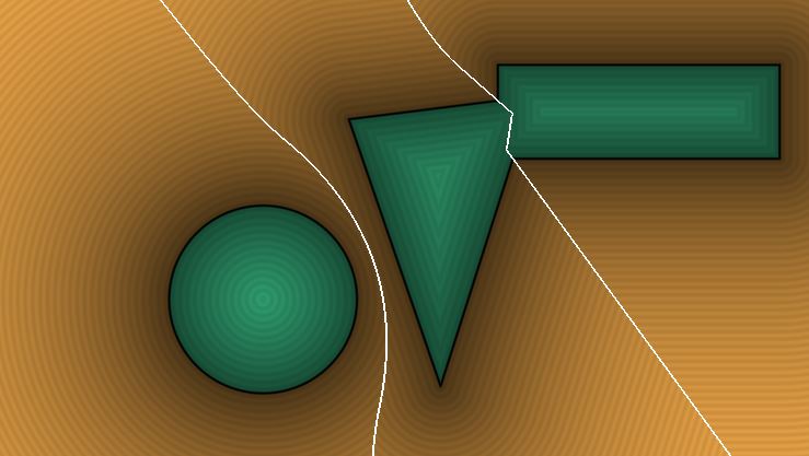
// Computes the laplacian of a distance field.
// The Laplacian measures average rate of change at a given location (while gradient measures
// the direction of maximum change). If compared agains a threshold, you can use is as an
// edge detector. You can also use it to detect linear sections of the distanec field, where
// the Laplace is zero, or alternativelly, measure how curved the isolines are (where the
// laplacian is higher the bigger the curvature).
float sdBox( vec2 p, vec2 b )
{
vec2 d = abs(p) - b;
return min(max(d.x,d.y),0.0) + length(max(d,0.0));
}
float sdTriangle( in vec2 p0, in vec2 p1, in vec2 p2, in vec2 p )
{
vec2 e0 = p1 - p0;
vec2 e1 = p2 - p1;
vec2 e2 = p0 - p2;
vec2 v0 = p - p0;
vec2 v1 = p - p1;
vec2 v2 = p - p2;
vec2 pq0 = v0 - e0*clamp( dot(v0,e0)/dot(e0,e0), 0.0, 1.0 );
vec2 pq1 = v1 - e1*clamp( dot(v1,e1)/dot(e1,e1), 0.0, 1.0 );
vec2 pq2 = v2 - e2*clamp( dot(v2,e2)/dot(e2,e2), 0.0, 1.0 );
float s = sign( e0.x*e2.y - e0.y*e2.x );
vec2 d = min( min( vec2( dot( pq0, pq0 ), s*(v0.x*e0.y-v0.y*e0.x) ),
vec2( dot( pq1, pq1 ), s*(v1.x*e1.y-v1.y*e1.x) )),
vec2( dot( pq2, pq2 ), s*(v2.x*e2.y-v2.y*e2.x) ));
return -sqrt(d.x)*sign(d.y);
}
vec2 v1, v2, v3;
float map( in vec2 p )
{
float d1 = length(p-vec2(-0.6,-0.3))-0.4;
float d2 = sdTriangle( v1, v2, v3, p );
float d3 = sdBox( p-vec2(1.0,0.5), vec2(0.6,0.2) );
return min( d1, min(d2,d3) );
}
void mainImage( out vec4 fragColor, in vec2 fragCoord )
{
vec2 p = (2.0*fragCoord.xy-iResolution.xy)/iResolution.y;
v1 = 0.7*cos( iTime*0.55 + vec2(0.0,1.5) + 0.0 );
v2 = 0.5*cos( iTime*0.50 + vec2(0.0,1.7) + 3.0 );
v3 = 0.8*cos( iTime*0.60 + vec2(0.0,1.6) + 4.0 );
vec2 e = vec2(2.0/iResolution.y,0.0);
float dis = map( p );
vec2 gra = vec2(map(p+e.xy)-map(p-e.xy), map(p+e.yx)-map(p-e.yx))/(2.0*e.x);
float lap = (map(p+e.xy) + map(p-e.xy) + map(p+e.yx) + map(p-e.yx) - 4.0*map(p))/(e.x*e.x);
//vec3 col = vec3(0.9+0.1*gra,0.0);
vec3 col = vec3(1.0,0.7,0.3);
if( dis<0.0 ) col = col.zxy;
col *= 1.0 - 0.7*exp(-1.5*abs(dis));
col *= 0.96 + 0.04*cos(200.0*dis);
col = mix( col, vec3(0.0,0.0,0.0), 1.0-smoothstep(0.0,0.01,abs(dis)) );
// laplacian display
float anim = fract( iTime/8.0 );
if( lap<-10.0 ) { if( anim>0.25 ) col = vec3(1.0,1.0,1.0); }
else if( lap> 10.0 ) { if( anim>0.50 ) col = vec3(1.0,0.8,0.1); }
else { if( anim>0.75 ) col += vec3(1.0,1.0,1.0)*abs(lap)*0.1; }
//col += vec3( abs(lap)*0.1 );
fragColor = vec4(col,1.0);
}
 Donate
No comments