Harmonic function: definitions and properties

Introduction
This is the second part of my tutorial series on bounded harmonic functions. For a quick introduction and examples of use of harmonic functions read the first part. In this part I define harmonic functions and their properties. This is the hard part with a lot of mathematics. But it's a mandatory step to understand how harmonic functions work. This will allow you to apply them in a broader context and understand many scientific papers relying on these. In addition this will be my entry point to introduce Finite Element Method in future posts. So hang on it's worth it!
Harmonic function definition and notations
In this section I will introduce the vocabulary and notions needed for the rest of the post.
So what is an harmonic function? It's a function \( f: \mathbb R^n \rightarrow \mathbb R\) which second derivatives sum to zero. So it must satisfy the equation:
\begin{equation} \frac{\partial^2f}{\partial x_1^2} + \frac{\partial^2f}{\partial x_2^2} + \cdots + \frac{\partial^2f}{\partial x_n^2} = 0 \label{eq:laplace} \end{equation}
Which for a 2D function \( f(x,y) \) would be \( \frac{\partial^2 f}{\partial x^2} + \frac{\partial^2 f}{\partial y^2} = 0 \) or \(f_{xx} + f_{yy} = 0\) depending on how you like to write your derivatives. This equation is a differential equation. However it is a special type of differential equation. Because \( f \) has multiples variables it is called a partial differential equation (PDE). Among the numerous PDEs the above equation is also named the Laplace equation.
I showed earlier how to compute with a diffusion process discrete harmonic functions. In these examples if you pick any point \( (x, y) \) then \( f(x,y) \) has to verify the Laplace equation \(f_{xx} + f_{yy} = 0\). We'll see every points do, even if for some it is not so obvious, but we'll get back on that.
What we have done using the diffusion process is: solving numerically the Laplace equation \(f_{xx} + f_{yy} = 0\) (a PDE) for every points of the grid. It is a numerical solution since the solution \( f \) is represented with a discrete grid of finite numerical values.
Values at the boundary are sometime called constraints, they're fixed. By opposition values inside the boundary (interior domain) are free or unknown.
Laplace operator
Usually the Laplace equation (\ref{eq:laplace}) is written using the Laplace operator denoted \( \Delta \). So the Laplace equation is equivalent to:
$$ \Delta f = 0 $$
\( \Delta \) is called a differential operator. Much like a minus sign '\( - \)' is applied to a value to negate it, differential operators are applied to functions and differentiate them. And so, \( \Delta = \frac{\partial^2}{\partial x_1^2} + \frac{\partial^2}{\partial x_2^2} + \cdots + \frac{\partial^2}{\partial x_n^2}\) and when applied \( \Delta f = \frac{\partial^2f}{\partial x_1^2} + \frac{\partial^2f}{\partial x_2^2} + \cdots + \frac{\partial^2f}{\partial x_n^2}\)
N.B: Laplace operator \( \Delta \) can be defined with the gradient \( \nabla \) and divergence \( \nabla \mathbf . \) (please notice the dot) differential operators:
$$ \nabla \mathbf . \nabla f = \Delta f $$
The gradient \( \nabla = \begin{bmatrix} \frac{\partial }{\partial x_1}, & \frac{\partial}{\partial x_2}, & \cdots &, \frac{\partial}{\partial x_n} \end{bmatrix} \) is a vector of first derivatives. for \( f: \mathbb R^n \rightarrow \mathbb R\) its dimension equal the number of arguments. So when applied we have: \( \nabla f: \mathbb R^n \rightarrow \mathbb R^n \).
The divergence \( \nabla \mathbf . \) (don't forget the dot) return a scalar value. It is meant to be applied to a vector field \( f: \mathbb R^n \rightarrow \mathbb R^n\):
$$f(x_1, \cdots, x_n) =
\begin{bmatrix}
f_1(x_1, \cdots, x_n) \\
\vdots \\
f_n(x_1, \cdots, x_n)
\end{bmatrix} $$
It computes \( \nabla \mathbf . f = ( \frac{\partial f_1 }{\partial x_1} + \frac{\partial f_2 }{\partial x_2} + \cdots + \frac{\partial f_n }{\partial x_n} ) \).
Some properties
The following will present some properties of harmonic functions. This will help you foresee and understand the shape of the function given a specific boundary condition.
Minimal surfaces
My preferred way to understand and predict the shape of an harmonic function is the analogy with soap bubbles or more precisely soap films:
 |
 |
 |
| Helicoid | Catenoid | Miscellaneous |
| Courtesy of © The Exploratorium. www.exploratorium.edu |
Courtesy of soapbubble.dk. (license CC BY-NC 3.0) |
Courtesy of math.hmc.edu |
The soap film have the particularity to be minimal surfaces. Depending on the structure the soap film is spread onto, the film shape will try to have the smallest possible surface in order to minimize the overall tension.
So what does it has to do with harmonic functions? Well minimal surfaces have their mean curvature null everywhere i.e they respect the Laplace equation (\ref{eq:laplace}). When you visualize in 3D a 2D harmonic function (see plots of previous chapter) you will see that indeed harmonic functions does seem to behave like the surface of soap films.
- Present an example of connected tubes with a membrane (Mario Botsh slides)
You like the analogy see this great video about minimal surfaces.
1D functions
Lets take a look at the solution of the Laplace equation in 1D to better understand how it behaves. In 1D we seek \( f : \mathbb R \rightarrow \mathbb R \) which satisfy \( f''(x) = 0 \). It isn't that hard to find out:
$$ \begin{eqnarray*} \iint f''(x) & = & \iint 0 \\ \int f'(x) & = & \int a \\ f(x) & = & ax + b \\ \end{eqnarray*} $$
This analytical solution tells us something interesting: 1D harmonic functions are always linear. This explains our earlier experiment:

when diffusing values on a 1D array it converges to a straight line. Another way to see it, is that a 1D function is a curve, and having \( f''(x) = 0 \) everywhere means it has no curvature, hence the straight line.
2D functions
The 2D version is a bit more tricky. To satisfy \(f_{xx} + f_{yy} = 0\) the obvious solution is for \( f \) to be linear in its principal directions \( x \) and \( y \). Indeed if \( f \) is linear in \(x\) and \(y\) directions then \( f_{xx} = 0 \) and \( f_{yy} = 0 \).
Here is an example of how to numerically compute such harmonic function, we simply set the boundary values on the top and bottom of the grid before applying a diffusion process (see previous chapter)

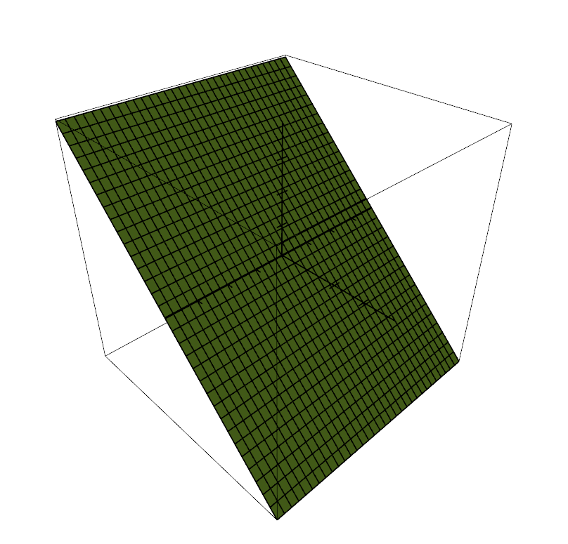
This perfectly illustrates the linear case. We can see that the variations of \( f \) from bottom-up is linear (visualized in 3D this is tilted plane). You can deduce from this observation that the functions of the form:
$$ f(x,y) = ax +by $$
Are all harmonic functions. Indeed every plane have a null mean curvature.
But this doesn't mean this is the only type of harmonic functions in 2D. The definition is \(f_{xx} + f_{yy} = 0\) not \( f_{xx} = 0 \) and \( f_{yy} = 0 \). So the other possibility is that the second derivatives \( f_{xx} \) and \( f_{yy} \) cancel each other out without individually being equal to zero. Take an analytical example such as \( f(x,y) = x^2 - y^2 \). Second derivatives are \( f_{xx} = 2 \) and \( f_{yy} = 2 \) and cancel out. This is a saddle function of the form:
$$ f(x,y) = ax^2 - by^2 $$
The saddle has two concavity with opposite orientation or opposite curvatures which cancels out. This is not the most practical example but it is good illustration for what follows. When \( f \) is harmonic and not linear then it has to have this saddle shape locally everywhere. This is the only way second derivatives can cancel each other out.
This bring us to the last example:

where it isn't so clear that \( \Delta f = 0 \) everywhere. Again here an analytical example can help: the function \( f(x,y) = \ln{ \sqrt{x^2 + y^2} } \) looks a lot like the last harmonic function presented in the previous chapter:

If you trust me on the computation of the second derivatives, they are as follows:
$$ f_{xx}(x, y) = \frac{-2x^2}{ (x^2 + y^2)^2 } + \frac{1}{x^2 + y^2} \text{ and } f_{yy}(x, y) = \frac{-2y^2}{ (x^2 + y^2)^2 } + \frac{1}{x^2 + y^2}$$
and do cancel each other out:
$$ \begin{eqnarray*} f_{xx} + f_{yy} & = & \frac{-2x^2}{ (x^2 + y^2)^2} + \frac{1}{x^2 + y^2} + \frac{-2y^2}{ (x^2 + y^2)^2} + \frac{1}{x^2 + y^2} \\ & = & \frac{-2(x^2 + y^2)}{ (x^2 + y^2)^2 } + \frac{2}{x^2 + y^2} \\ & = & \frac{-2}{ x^2 + y^2} + \frac{2}{x^2 + y^2} \\ & = & 0 \end{eqnarray*} $$
TODO: unfortunately this tutorial is still work in progress. I'll leave the outline here as a reminder for me and for your reference, who knows it my help you.
The maximum principle
The maximum principle states that a non-constant harmonic function cannot attain a maximum (or minimum) at an interior point of its domain. This result implies that the values of a harmonic function in a bounded domain are bounded by its maximum and minimum values on the boundary. In other words: "no interior local extrema in f"
Uniqueness Principle:
If we know the values of the function along the boundary of a region, there is only one harmonic function defined in that region with those boundary values.
mean-value property
"it streches"
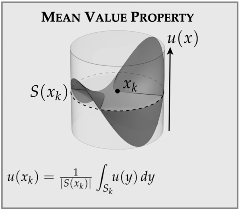
The value at any point \( x_k \) is equal to the average value over any sphere around that point.
On a 2D domain (hot plate examples the average temp on the border of a circle is the same at its center):
\[ u(x_k) = \frac{1}{2} \int_0^{2\pi} { u(x_k + r e^{i \theta}) d \theta } \]Hot plate illustration:

Boundary continuity
C0
(todo: image C0 function, mesh deformation)
Dirichlet energy
The Dirichlet energy is a measure of how variable a function is. It's defined as:
\[ E[u] = \frac 1 2 \int_\Omega \| \nabla u(x) \|^2 \, dx \]
with:
- \( \Omega \in \mathbb R^n \) an open set
- \(u : \Omega \rightarrow \mathbb R\) a scalar function
An harmonic function (i.e. that respect the Laplace equation \( \Delta u = 0 \)) minimizes the Dirichlet energy!
Summary
- give the equation with laplace operator
- give some properties of harmonic functions
- (linear along the principal directions)
- C0 on the boundary (give 1D example with three constrainsts and 2D example shown in 3D)
- maximum principals?
The computation of the interior will be done by solving a linear system:
$$ \mathbf A \mathbf x = \mathbf b$$
Where the unknown \( \mathbf x \) are the values of \( f \) at every points of the 2D grid. I shall describe \( \mathbf A \) and \( \mathbf b \) in the next sections.
Solving the Laplace equation
Introduction
- explain It's a PDE
- PDE can be solved on discrete domains like grids
- it's called FDM
- we can use triangles teghtrahedral but its FEM and need to redefine Laplace operator
- Give link books on PDE
Setup the linear system
- For a nXn grid there is n*n unknown
- the system is:
- Give the stencil and finite difference
- Give the laplacian matrix for 2D grid
- PDF laplacian matrix regular grid summary with stencil finite diff and matrix for 1-2-3D
- Setup the constraints
- Code to fill the matrix
Solving the system
Diffuse values with Gauss-Seidel
- 1D example
- 2D case
- Code to solve
Multi grid approach
LU decomposition
Code to solve
LLT decompostion
Code to solve
References
 Donate
No comments