[Summary] Weak Formulation For Finite Element Analysis
$$ % This version will make mathjax ignore the width of the annotation and keep the main % formula centered. Obviously this mean the annotation is forcefully placed to the right % and may bleed out: \newcommand{Annotation}[1]{ \rlap{~~~~~~\raise 0.8em {\color{grey}\scriptsize{ #1 }}} } \newcommand{annotation}[1]{ {~~~~~~\raise 0.8em {\color{grey}\scriptsize{ #1 }}} } $$Strong form
Poisson equation PDE:
$$ u''(x) = f(x) $$boundary conditions for the PDE $u(0)=0$, $u'(1) =0$
Weak form:
$$ \int u'(x)v'(x) = [u'(x)v(x)] - \int f(x)v(x) \ \ dx \ \ \text{ for all } v(x) $$$v(x)$ is called the test function and can be any function.
$$ \begin{aligned} u''(x) &= f(x) \\ u''(x)v(x) &= f(x)v(x) \\ \int_a^b u''(x)v(x) &= \int_a^b f(x)v(x) \\ [u'(x)v(x)]_a^b - \int_a^b u'(x)v'(x) \ \ dx &= \int_a^b f(x)v(x) \annotation{ \text{partial integration} \\ \text{of left hand side} } \\ \end{aligned} $$Set integral range to $[0,1]$, and with boundary conditions for the PDE $u(0)=0$, $u'(1) =0$ and forcing the test function to respect $v(0) = 0$:
$$ \begin{aligned} u'(1)v(1) - u'(0)v(0) - \int_a^b u'(x)v'(x) \ \ dx &= \int_a^b f(x)v(x) \\ - \int_a^b u'(x)v'(x) \ \ dx &= \int_a^b f(x)v(x) \\ \end{aligned} $$Transcripts
This is a transcript of the video https://www.youtube.com/watch?v=xZpESocdvn4 all images and text are all properties of the original author
The weak formulation! You probably stumbled over this term already in one of your classes on finite elements or partial differential equations, and perhaps you had problems understanding where the weak formulation comes from and why it is so useful.
In this video we will take a close look at the weak formulation and visually explore its properties. If you never heard about the weak formulation before, don't worry, we will start from the very beginning here.
Many problems in physics or engineering can be described by differential equations, which we want to solve for an unknown solution function.
$$ u''(x) = f(x) $$ Here you see differential equation in its conventional form, which is called the strong form, we will see later why. Transforming differential equations from their conventional form into what is called their weak form is nowadays an indispensable tool when it comes to numerically solving differential equations. $$ \int u'(x)v'(x) = [u'(x)v(x)] - \int f(x)v(x) \ \ dx \ \ \text{ for all } v(x) $$However, just from looking at the formulas, it is not quite easy to understand the concept concept of the weak formulation.
Why are there other functions than our unknown solution function in the weak formulation?
$$ \int u'(x){\color{red}v'(x)} = [u'(x){\color{red}v(x)}] - \int f(x){\color{red}v(x)} \ \ dx \ \ \text{ for all } v(x) $$ What does it mean that the weak formulation has to hold true for all of these functions? $$ \int u'(x)v'(x) = [u'(x)v(x)] - \int f(x)v(x) \ \ dx \ \ \color{red} \text{ for all } v(x) $$And why is it even called weak formulation? These questions will be addressed in this video and we will explore why the weak formulation is so incredibly useful for solving differential equations with the finite element method (FEM). And I promise you: once having understood the weak formulation understanding the finite element method will be comparatively easy.
The strong formulation
But let's start from the very beginning. Before we talk about the weak formulation let's take a look at the differential equation in its conventional form: the strong formulation.
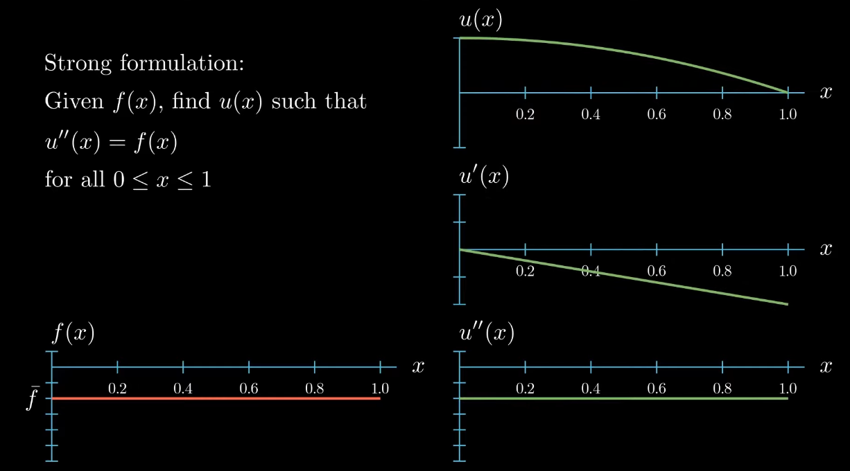
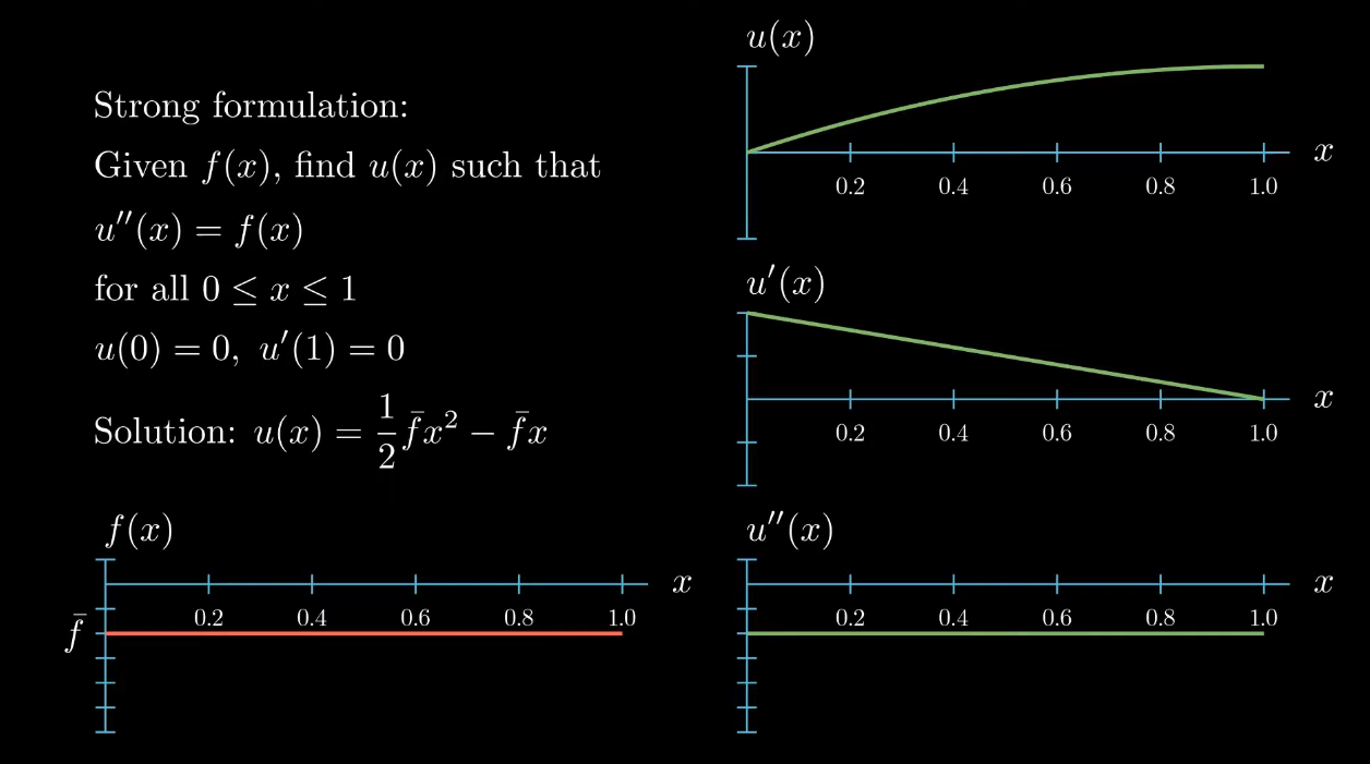
In this video we will take a look at the arguably most popular differential equation: the Poisson equation. This differential equation is so popular because it naturally appears in many scientific applications. The strong formulation of the Poisson problem in 1D states that for a given function $f(x)$ find a function $u(x)$ such that its second derivative which is here denoted by u'' is equal to f(x).
$$ \begin{aligned} \text{Given } f(x) \text{, find } u(x) \text{ such that}\\ u''(x) = f(x) \end{aligned} $$So we want to find the function $u$ whose second derivative is $f$. Typically we are only interested in how this function looks like on a specific region of interest. Here I'm choosing the interval $0 \leq x \leq 1$.
$$ \begin{aligned} \text{Given } f(x) \text{, find} u(x) \text{ such that}\\ u''(x) = f(x) \\ \text{for all } 0 \leq x \leq 1 \end{aligned} $$Let's visualize this. We are interested in the function $u$ of $x$. How does function looks like is not known.
Here I'm just illustrating an exemplary function.
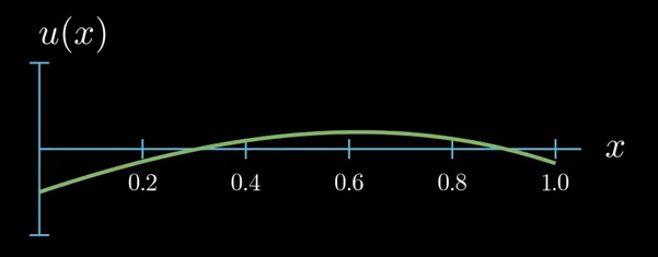
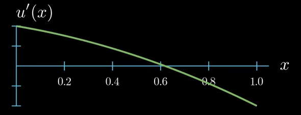
As you know the derivative of u describes the slope of $u$ at each point $x$
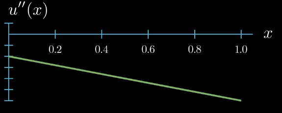
and the second derivative which appears in our differential equation describes the slope of the slope of $u$ which can also be interpreted as the curvature of $u$.
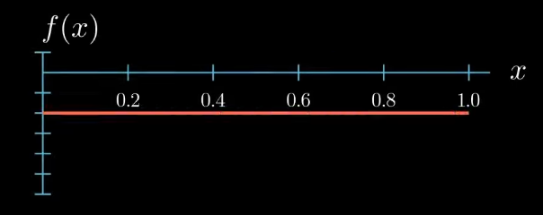
We have given a function $f$ of $x$. In this video I will assume that $f(x)$ is constant taking the same value at each point $x$. I will denote this value by $f$ bar.
Our differential equation states that we want to find the function $u$ such that its second derivative is equal to $f$. Here I'm illustrating an exemplary function whose second derivative equals $f$:
So this function is a solution to our differential equation. Notice however that moving the function u up and down
has no influence on the slope and no influence on the curvature of $u$, likewise "rotating" (What I really mean here is that adding a linear function to u does not change its curvature. If the linear function is ax + b and if a is small, adding this function to u looks a bit like rotating u.) $u$ does change the slope of $u$ but again it does not have an influence on the curvature of $u$.
Therefore we could find infinitely many functions $u$ that fulfill our given differential equation. To avoid this we add boundary conditions to our problem. Here I will assume that $u$ at $x = 0$ is $0$ and the first derivative of $u$ at $x = 1$ is $0$.
$$ \begin{aligned} \text{Given } f(x) \text{, find} u(x) \text{ such that}\\ u''(x) = f(x) \\ \text{for all } 0 \leq x \leq 1 \\ u(0) = 0, u'(1) = 0 \end{aligned} $$There's only one function that fulfills the differential equation and the boundary conditions at the same time. For this very simple one-dimensional example we can even find an analytical expression for this function. We obtain this quadratic expression for $u$.
$$ u(x) = \frac{1}{2} \bar fx^2 - \bar f x $$By plotting $u$ and its derivatives we observe that $u$ indeed fulfills the differential equation because the second derivative of $u$ equals $f$ and $u$ indeed fulfills the boundary conditions because $u$ is $0$ at $x = 0$ and $u'$ is $0$ at $x = 1$.
Note however that deriving such analytical expressions for our solution is only possible for very simple differential equations. In general the solution to the differential equation may not be so easy to compute by hand hand and we have to rely on computer algorithms for finding the solution function $u$ or sufficiently good approximations of it.
5:10
The so-called finite element method is one of the most popular methods for solving differential equations numerically. The idea of the finite element method is to split our region of interest into a number of segments.
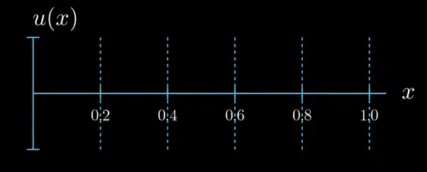
These segments are called elements and the points between the segments are called nodes. Next, we formulate a set of very simple functions which are respectively one at one node and zero at the other nodes.
These functions are called shape functions. As we have six nodes in this example there are six shape functions $N_i$. The index $i$ of $N_i$ indicates to which node a shape function belongs to.
Finally we assume that our solution function can be expressed as the sum of the shape functions multiplied by a set of parameters which are here denoted by $u_i$.
$$ u(x) = \sum_{i=0}^5 u_i N_i(x) $$These parameters can take arbitrary values. If we set all of them to zero, our solution function is zero. By tweaking the parameters we obtain differently shaped functions $u$
Note that by assuming that our solution can be expressed as the sum of simple functions multiplied by tunable parameters, that is by introducing a parametric "ansatz" for our solution (I am using the word ansatz for the assumed form of the solution function u. Although ansatz is a German word, it is also frequently used in English, especially in the mathematical context.), we have reformulated the problem of finding an unknown function into a problem of finding a set of unknown parameters. Such problems can be handled much better by computers. But how could we possibly find out which values the unknown parameters should take?
The naïve approach would be to substitute our assumed expression for the solution function into the differential equation and see if we can solve for the unknown parameters.
$$ \begin{aligned} \Biggl ( \sum_{i=0}^5 u_i N_i(x) \Biggr )''(x) = f(x) \\ \text{for all } 0 \leq x \leq 1 \\ u(0) = 0, u'(1) = 0 \end{aligned} $$But there is a catch! This naïve strategy is not possible which becomes clear immediately after looking at how the second derivative of our solution function looks like.
Ignoring the points at which our function is not differentiable we see that the second derivative of $u$ is zero everywhere and this does not change upon changing the values of the unknown parameters. This means that there is no possible combination of parameters such that the strong formulation of the differential equation is fulfilled. We arrived at the dead end. We have introduced a parametric ansatz for our solution function but we cannot substitute it in the differential equation to compute the unknown parameters in our ansatz.
Therefore we need to reformulate our problem into a form that is more suitable to be solved with the finite element method . We need to transform the strong formulation into what is called the weak formulation of the problem
8:11
The Weak Formulation
So let's talk about the weak formulation. In what follows we will derive the weak formulation from the strong formulation and for the next few minutes please do not focus on why we are doing this but rather focus on why we are mathematically allowed to reformulate the problem like this. The usefulness of the weak formulation will become apparent later.
First we write down the problem in the strong form.
$$ u''(x) = f(x) $$Next we introduce a type of functions which we call test functions $v(x)$. The test functions are like $u(x)$ defined on an interval between x equals 0 and 1 and they may take any arbitrary shape on this interval.
Now we multiply both sides of the differential equation by these test functions.
$$ u''(x)v(x) = f(x)v(x) $$This is a valid mathematical operation because we apply the same manipulations on both sides of the differential equation. If $u''$ is equal to $f$ then also $u'' \times v$ must be equal to $f \times v$.
Afterwards we integrate both sides of the differential equation over our region of interest that is from $x = 0$ to $x = 1$.
$$ \int_0^1 u''(x)v(x) = \int_0^1 f(x)v(x) $$Once again this is a valid mathematical operation because we are applying the same manipulations on both sides of the equation. Note now, that we can apply these manipulations on both sides of the differential equation for any arbitrarily chosen test function $v$. No matter how we choose $v$ our newly derived integral equation must hold true. Therefore we write that the integral equation must hold true for all test functions $v$.
Finally like the strong formulation the weak formulation must fulfill the boundary conditions. That's it. $$ \begin{aligned} & \int_0^1 u''(x)v(x) = \int_0^1 f(x)v(x) \\ & \text{for all } v(x) \\ & u(0) = 0, \ u'(1) = 0 \\ \end{aligned} $$We have derived the weak formulation from the strong formulation by multiplying both sides of the differential equation by the test functions and integrating both sides of the equation over the region of interest.
However are we really allowed to do this?
Whenever we manipulate an equation we must be very careful not to lose any information that the equation provides us. So the natural question that arises is whether we can recover all information that the strong form provides us from the weak form. In other words: we know that we can derive the weak form from the strong form but can we likewise derive the strong from the weak form? In the following we will try to answer this question by visually exploring the weak formulation.
Let's take a look at the weak formulation and let's focus on the right hand side of the equation
$$ \int_0^1 u''(x)v(x) = \color{red} \int_0^1 f(x)v(x) $$first the function $f(x)$ is given we have assumed that it takes a constant value $\bar f$
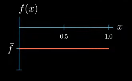
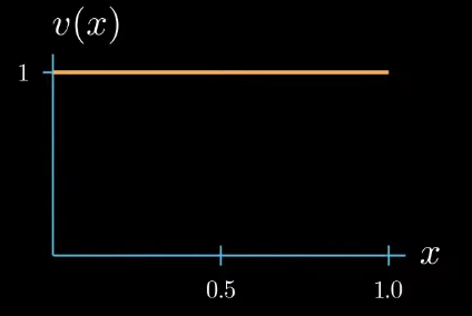
the test function $v(x)$ is arbitrary the weak formulation must hold true for all test functions that we could think of so we can choose any shape for the test function here
but let's choose a test function with a constant value of 1 for now
next let's plot $f \times v$.
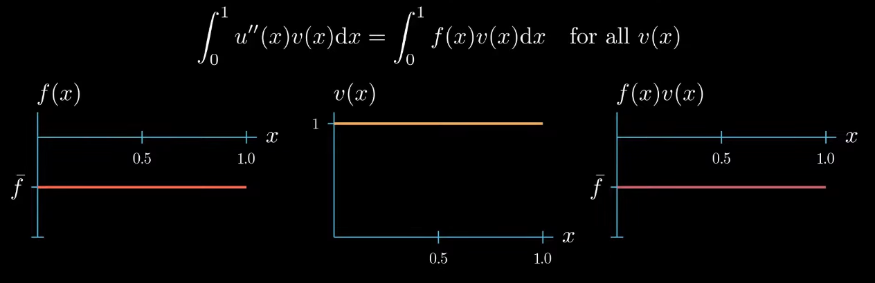
Multiplying two functions is a pointwise operation that means for every point $x$ we multiply the corresponding values $f(x)$ and $v(x)$ as $f$ is constantly taking the value $\bar f$ and $v$ is constantly 1. $f \times v$ is again a constant function that takes the value $\bar f$.
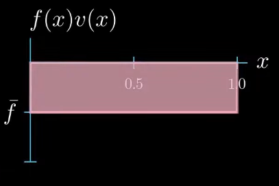
note that the right hand side side of the weak form is the integral of $f \times v$ from $0$ to $1$ which describes this area here.
Now let's move on to the left hand side of our equation.
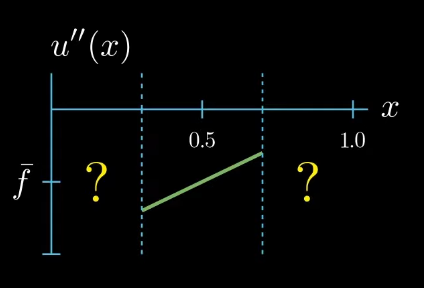
$$ {\color{red} \int_0^1 u''(x)v(x)} = \int_0^1 f(x)v(x) $$ The second derivative of $u$ is unknown because $u$ is our unknown. The test function is the same as on the right hand side of the equation, which we have arbitrarily chosen as constantly $1$ for now. Finally the second derivative of $u$ times the test function $v$ is also unknown, because the second derivative of $u$ is unknown so the second derivative of $u$ times the test function $v$ can be a function of arbitrary shape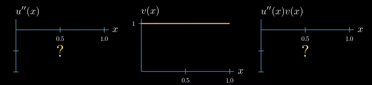
however there's one constraint the weak formulation tells us that the integral of $u'\times v$ must be equal to the integral of $f \times v$ therefore this area must be equal to this area
this means that $u'' \times v$ can take arbitrary shapes as long as the area is preserved for example this shape is allowed or this shape or this shape
knowing that $\int u'' v = \int vf$ what does this tell us about $u''$?
In this particular example we have chosen a test function that is constantly one this means that $u'' = u''v$, but we can see that choosing the test function as constant does not provide us much information about how $u''$ looks like. $u''$ can take any shape as long as $\int u''v = \int fv$.
We can conclude that by choosing a test function of constantly 1, we force the integral of $u''$ to be equal to $\int f$, however, we don't obtain any further information about how $u''$ should look like. That being said, the weak formulation must hold true for any test function $v$, so let's see if we can construct a test function that is more useful for getting information about how $u''$ looks like.
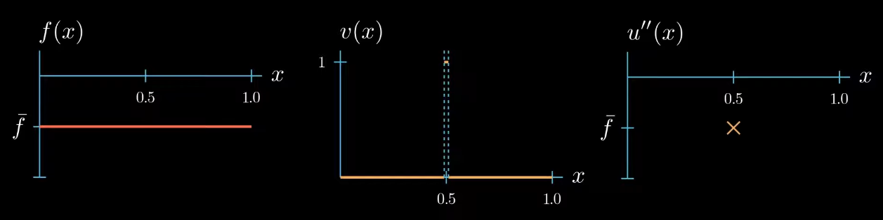
Let's start with a test function that is 1 over an interval $I$ and 0 elsewhere.
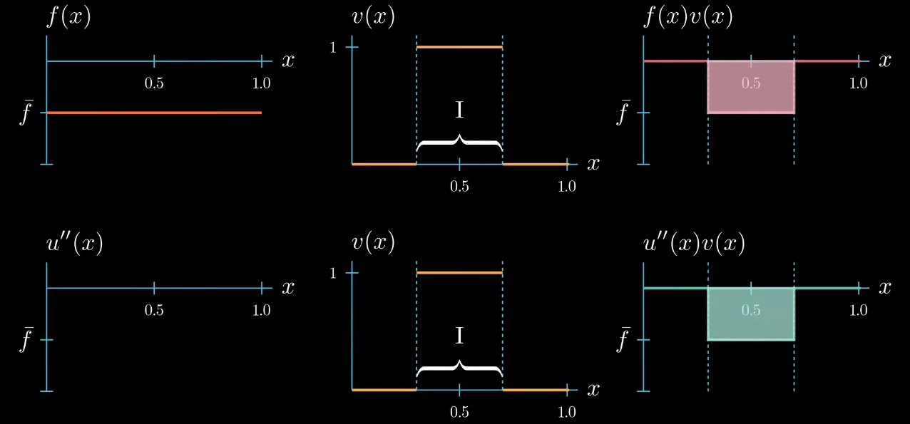
$fv$ is now a function that is equal to $\bar f$ over the interval $I$ and 0 elsewhere. We also know that $u''v$ must be 0 outside the interval $I$ because $v$ is 0 there. Inside the interval the shape of $u''v$ is unknown, we only know that its integral is equal to $\int fv$ (same area).$
Because $v$ is constantly 1 over the interval $I$, we know that $u''$ and $u''v$ are equal over the interval $I$.
But we do not know how $u''$ could look like outside the interval $I$
On the first glance it seems that we did not gain any new information about how $u''$ should look like after changing the shape of our test function. But let's take a closer look if we assume that $u''$ is a continuous function, which we will do here. We can observe that $u''$ must cross at some point in the interval $I$ the value $\bar f$, even if we change the shape of $u''$ crosses $\bar f$ at least once.
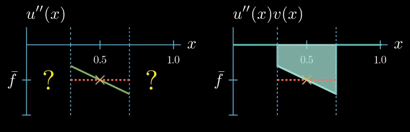
this is because otherwise the area under $u''v$ cannot be equal to the area under $fv$.
Now this is a useful information we have chosen the test function $v$ such that we know that $u''$ takes the value $\bar f$ somewhere in the interval $I$. We just don't know where exactly.
but let me remind you once more the weak formulation must hold true for any test function therefore we can decrease the interval $I$ over which our test function is chosen to be equal to 1. By doing so we narrowed down the interval in which we know that $u''$ is equal to $\bar f$... Can you see where this is going! We can decrease the interval even further, and in the limit, we will see that we are very certain about where u'' must take the value $\bar f$.
Let's step back for a second and see what we have achieved. By choosing a specifically designed test function we found that $u'' = \bar f$ at one point $x$.
Because the weak formulation must hold true for any test function we can repeat the same argument to find that $u'' = \bar f$ at another point $x$ let's see what happens if we repeat this argument a couple of times
 Donate
No comments