How to generate bounded harmonic weights on a regular grid
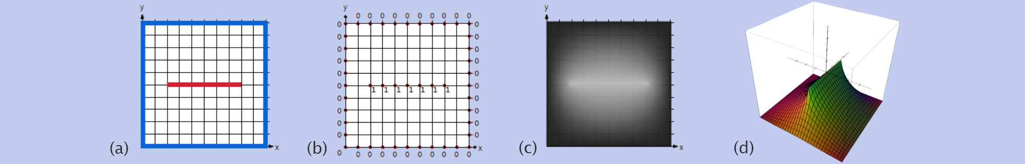
Generating an height-map is a good example to demonstrate how useful harmonic functions can be. In (a) user can stroke lines corresponding to different heights. In (b) we associate a height where the strokes lies. In (c) we compute the rest of the values automatically (black is zero, white is one). (d) is a 3D view of the heightmap in (c). It is a 2D function \( f: \mathbb R^2 \rightarrow \mathbb R\) which returns the height. The tutorial explains how to compute the unknown heights and ensure \(f\) is an harmonic function.
Summary
In this tutorial I give the basics to be able to compute harmonic functions \( f: \mathbb R^n \rightarrow \mathbb R\) over a regular grid/texture (in 1D, 2D or 3D). All you need is to set a few values on the grid that define a closed region (see figure above), then the remaining values are automatically computed using the so-called Laplace operator and solving a linear system of equations. After a quick and "mathless" presentation of an easy way to implement this in C++, I will explain the mathematical jargon. This tutorial is the first of series which will lead to more complicated techniques like Finite Element Methods (FEM).
Introduction
A practical example in 2D
Our goal is to generate a 2D function \( f: \mathbb R^2 \rightarrow \mathbb R\) discretized and stored in a 2D array array[x][y] = f(x,y):
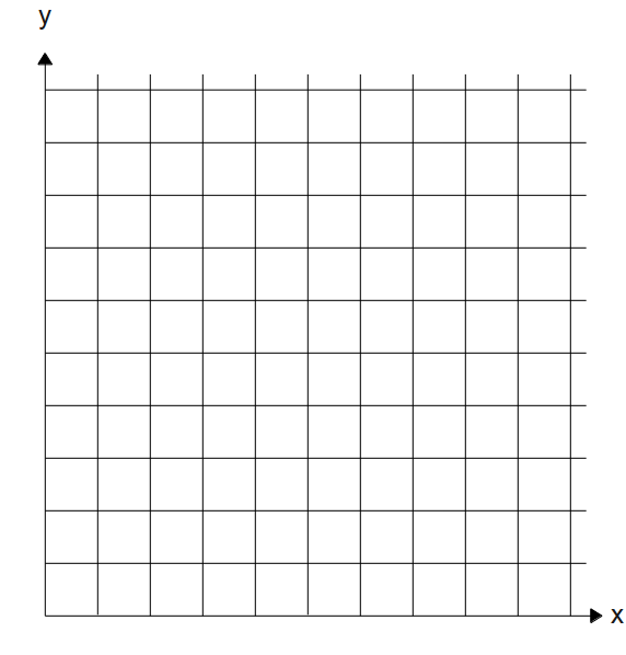
First we set by hand some values of the grid. These values must form a closed boundary, here is an example of such closed region:
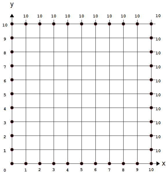
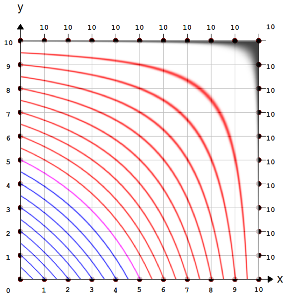
Note that the boundary doesn't necessarily have to lie on the border of the grid. We could define the closed region as a circle, rectangle or even a free-form curve. A closed boundary will guarantee we can compute values inside the domain. This is what \( f \) looks like when we apply the algorithm (presented later in this article) on the above boundary conditions:
 |
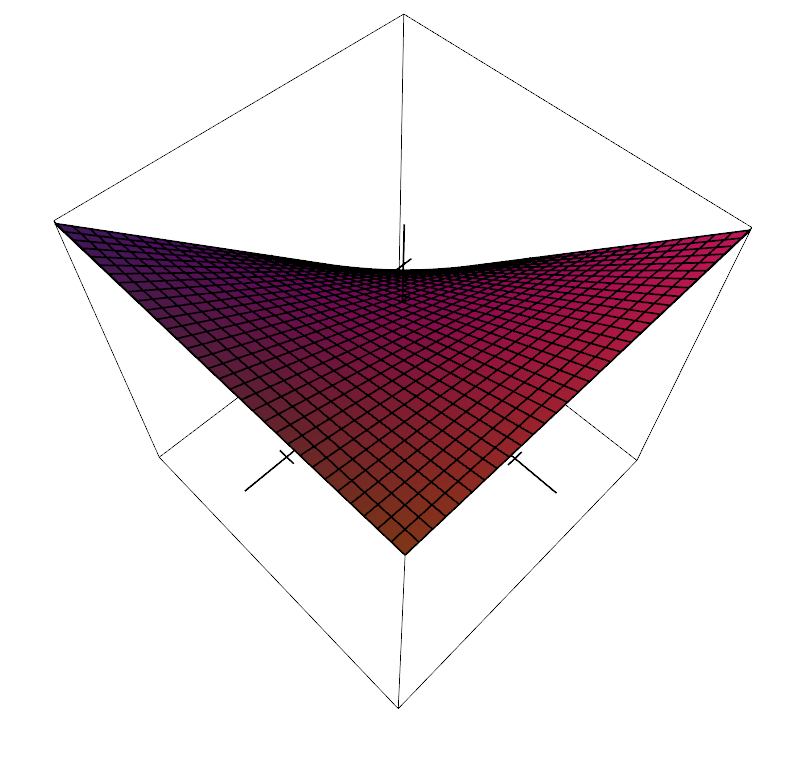 |
| values of \( f(x, y) \) are shown with level curves. The curves colors mean: 5 for Pink, below 5 blue, above 5 red and black for 10. | The same plot of \(f\) but in 3D (view from top). |
Here \(f\) is harmonic: the function respects certain properties and will always have the same shape for a given closed boundary.
The function \( f \) is called differently depending on the context. In mathematics we refer to it as a scalar-function or scalar-field. Indeed the function associates a point in space \( \mathbf p \) (2D, 3D etc.) to a scalar (i.e a single real number). When \( f \) returns a height like the introductory example we may call it a height-field. Sometimes \( f \) is called a weight-map as it maps every points of the plane/volume/etc. to a weight (real number).
Before diving into the technicalities, lets see how all this is useful in the realm of computer graphics.
Motivation
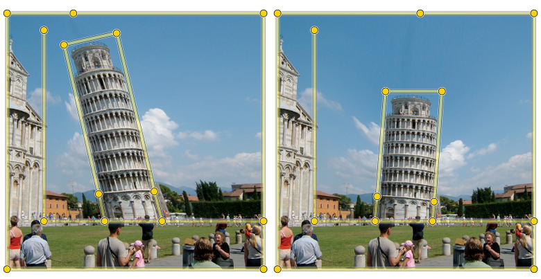
Being able to compute weight maps by only specifying a few values on a canvas is extremely useful. Besides height maps there are tons of applications where you need to generate such smooth transition of values / smooth shade over a surface. For instance, cage deformation, where you enclose an object into a cage and deform it by moving the cage's vertices:
 |
 |
 |
| A circle in a cage in rest pose. | When moving the cage's vertex we deform the circle. | The influence of one vertex of the cage. Blue means full influence. This influence is defined as an harmonic function. |
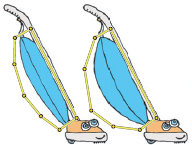
Here are more concrete examples of such deformation:
 |
 |
|
(These examples actually use bi-harmonic functions but the idea is the same) |
|
If you want to understand how these weight maps are used to deform objects, you can find here a nice essay introducing harmonic coordinates specifically for cage-based deformations (the article doesn't go as far as I plan to do though).
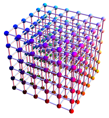
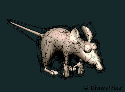
Although I have only presented 2D examples on regular grids, harmonic functions can be computed on various domains. For instance cage deformations can be extended to 3D. On a regular 3D grid we can define an harmonic function \( f: \mathbb R^3 \rightarrow \mathbb R\). This function will tell the influence inside a triangular 3D cage:
 |
 |
 |
| We can compute an harmonic function \( f: \mathbb R^3 \rightarrow \mathbb R\) inside a 3D grid | A triangular cage defines a closed boundary inside this 3D grid. From there we can compute a weight map (or region of influence) for each cage's vertex. | Result of the deformation with 3D harmonic functions. |
Not only can we use regular grids (may it be 2D or 3D), we can also compute these harmonic functions over irregular domains like triangular meshes:
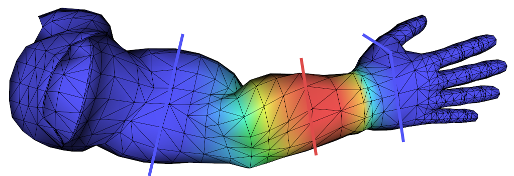 |
In this case the function is 2D \( f: \mathbb R^2 \rightarrow \mathbb R\) and defines a weight for each vertex of the triangular 3D mesh. Here I represented the boundaries with red and blue lines. The function \( f \) returns 1 at red vertices and decays towards zero at blue vertices. This can be particularly useful to define the so called skinning weights needed to animate a character. (note: computing skinning weights with harmonic functions is briefly described in context aware deformation section 2.2)
The diffusion algorithm
Back to our simple 2D problem. We would like to automatically compute values inside the closed boundary of our 2D rectangular grid. To this end we use a process called diffusion, the algorithm is quite simple:
- INITIALIZE( nodes ) // init every node of the grid (inside the boundary) to a value (usually 0)
- FOR( nb_interations ) // some arbitrary number
- FOREACH( node ) // look up nodes (e.g from left to right and bottom-up) of the grid
- Compute the average value of the four neighbors
- Replace the current node's value with the average
- FOREACH( node ) // look up nodes (e.g from left to right and bottom-up) of the grid
The idea is that each time you look up the grid and compute the average, the values from the boundary "leaks out"/diffuse to their direct neighbors. The more you repeat the process the more the values propagate inside the domain until it stabilizes. I always found amazing the fact that, if you don't change the values at the boundaries then what is inside will eventually converge to a steady state. For the same boundary values, you will always get the same values inside if you iterate enough this averaging process. In other word given a boundary, you always find a unique harmonic function \( f \) (if it exists). Here we found this function using the diffusion algorithm, but I will explain other ways in a couple of sections.
The C++ procedure below compute nb_iter iteration of the diffusion algorithm for the 2D case:
/// (untested code)

bool inside(const Grid_2d& grid, Vec2i idx)
{
    return idx.x() < grid.size().x() && idx.x() > -1 &&
           idx.y() < grid.size().y() && idx.y() > -1
}

/// @param grid : 2d grid of float values you want to diffuse
/// @param mask : 2d grid where values set to '0' means don't diffuse this position
void diffuse(Grid_2d& grid, const Grid_2d& mask, int nb_iter)
{
    assert(grid.size() == mask.size());

    // First we store every grid elements
    // that need to be diffused according to 'mask'
    int mask_nb_elts = mask.size().product();
    std::vector idx_list;
    idx_list.reserve( mask_nb_elts );
    for (int x = 0; x < mask.size().x(); ++x) {
        for (int y = 0; y < mask.size().y(); ++y) {
            if (mask(x, y) == 1)
                idx_list.push_back(Vec2i(x, y));
        }
    }

    // Diffuse values with a Gauss-seidel like scheme
    for (int i = 0; i < nb_iter; ++i)
    {
        // Look up grid elements to be diffused
        for (unsigned j = 0; j < idx_list.size(); ++j)
        {
            Vec2i idx         = idx_list[i];
            float sum         = 0.f;
            int nb_neighbours = 0;

            Vec2i above = idx + Vec2i( 0,  1);
            Vec2i below = idx + Vec2i( 0, -1);
            Vec2i left  = idx + Vec2i(-1,  0);
            Vec2i right = idx + Vec2i( 1,  0);
            if( inside(grid, above) ) { nb_neighbours++;  sum += grid(above.x(), above.y()) }
            if( inside(grid, below) ) { nb_neighbours++;  sum += grid(below.x(), below.y()) }
            if( inside(grid, left ) ) { nb_neighbours++;  sum += grid( left.x(),  left.y()) }
            if( inside(grid, right) ) { nb_neighbours++;  sum += grid(right.x(), right.y()) }

            float average = sum / (float)nb_neighbours;
            grid(idx.x(), idx.y()) = average;
        }
    }
}
The 1D case
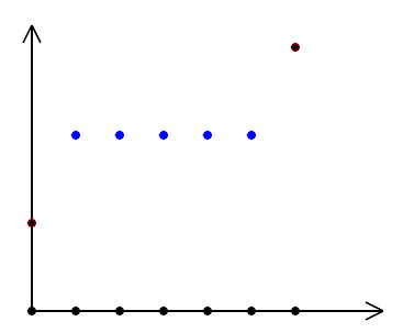
Diffusion works in \( nD \) and we can try it out on a \( 1D \) function to better see what is happening. Begin to store a function \( g : \mathbb R \Rightarrow \mathbb R\) in a one dimensional array. The array is initialized to zero except for the first and last elements (for instance: array[0] = 1.0 and array[size-1] = 3.0). Then we apply the diffusion by looking the array from beginning to end and compute the average ( array[i-1] + array[i+1]) / 2.0:
 |
 |
| Plot of \( g \) before diffusion | The diffusion process for every iterations until convergence. |
Again \( g \) converge to an harmonic solution.
Initial values
The grid must be initialized to some initial value/initial guess before diffusion. The choice of this starting point will impact the rapidity of convergence. If choose wisely this can drastically speed up the diffusion by decreasing the number of iterations needed:
 |
 |
| Before diffusion | The diffusion converge faster than above |
The 3D case
Extension to 3D grids is trivial, the boundary must define a closed volume (as opposed to a closed area in 2D) and the diffusion now average the 6th neighbors instead of the 4th neighbors in 2D. The number of iterations before it stabilizes will be extremely important as there is comparatively more grid's nodes for 3D than in 2D. Note that the diffusion algorithm is the slowest method to compute Harmonic functions. I will introduce more efficient methods afterwards.
More examples
Here I show more examples of harmonic functions for different boundary conditions:
 |
 |
 |
 |
| Boundary conditions and associated harmonic function \( f: \mathbb R^2 \rightarrow \mathbb R\) plotted with level-curves. | The harmonic function in 3D view |
In the second example notice that we can add fixed values inside the boundary as well.
Evaluate \(f\)
So far I have described how to compute a harmonic function at the location of the nodes of a grid, but what about values in between those nodes? For instance in the 1D case you may know the values \(f(1), f(2), \dots, f(n)\), but how can you compute \( f(0.6) \)? Well you need to interpolate the values of the nodes. You may choose the nearest value to \(f(0.6)\), a linear interpolation, cubic interpolation etc. For 2D grids bi-linear interpolation and 3D grids tri-linear interpolation.
Conclusion
We have seen how to compute harmonic functions over regular grids in 1D, 2D or 3D with the diffusion process. I also gave some examples of usage like cage-based deformations or height-maps. In the next tutorial we will talk about their mathematical properties. Knowing and understanding these properties will be very useful to use them correctly or compute them more efficiently (the diffusion process is the slowest way to compute harmonic functions).
 Donate
No comments