Compute Harmonic weights on a triangular mesh

Here I describe the discrete Laplace-Beltrami operator for a triangle mesh and how to derive the Laplacian matrix for that mesh. Then I provide [ ![]() C++ code ] to compute harmonic weights over a triangular mesh by solving the Laplace equation.
C++ code ] to compute harmonic weights over a triangular mesh by solving the Laplace equation.
Motivation
The goal here is to present the Laplace operator with a concrete application, that is, computing harmonic weights over a triangle mesh. In geometry processing the Laplace operator \( \Delta \) is an extremely powerful tool. For instance it can be handy to compute or process weight maps.
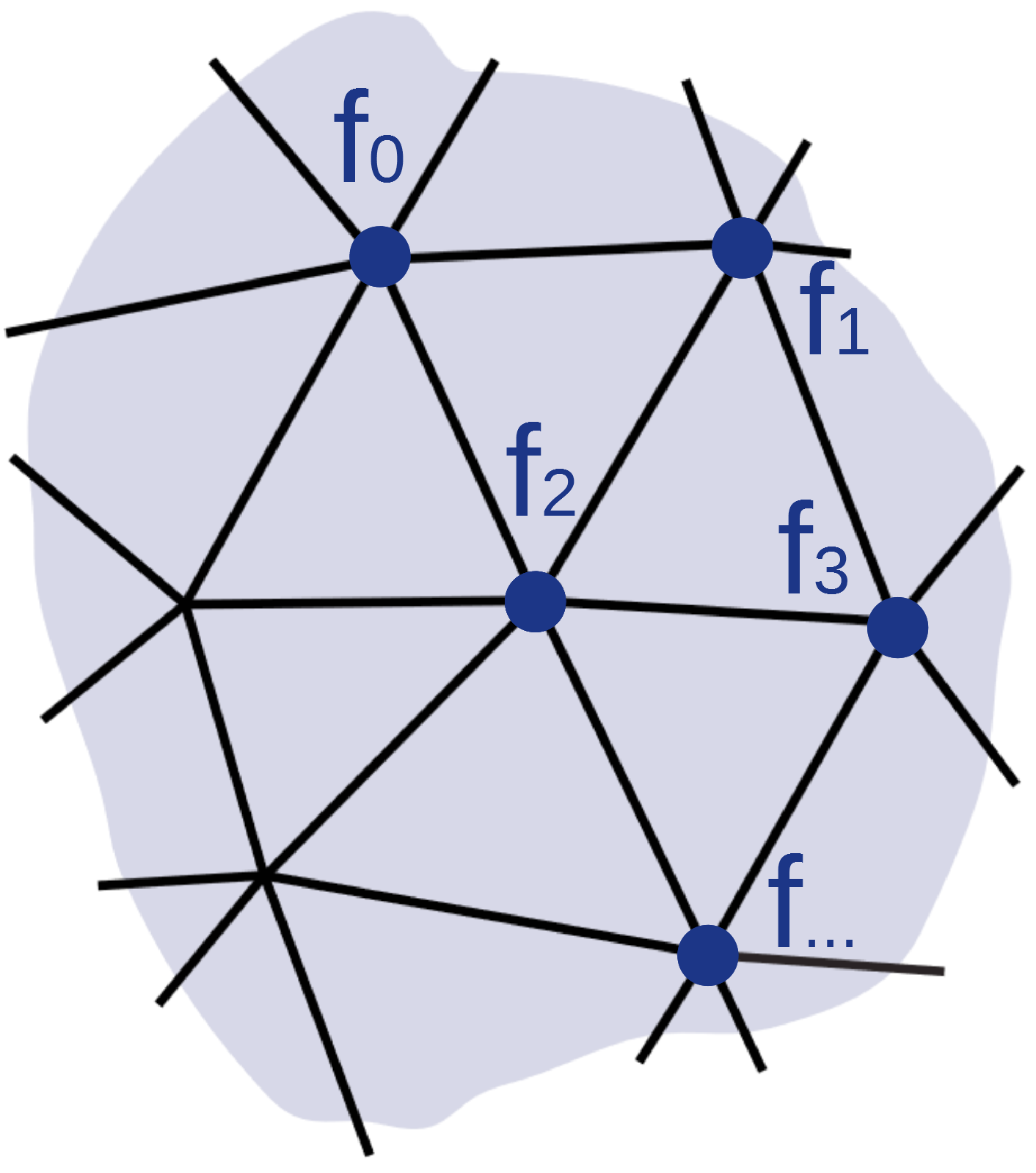
A weight map is a function \( f(u, v) \) that associates a point of a surface to a real value \( f(u, v): \mathbb R^2 \rightarrow \mathbb R\). Usually the weight map is discrete, meaning if our surface is represented with triangles and vertices, we can associate each vertex to a single scalar value (\(f_0=0.1\), \(f_1=-0.3\) etc ):
There are numerous occasion where you would want to associate some weight to your vertices, like setting a mass to each vertex for physic simulations, a height to create wrinkles like in bump maps, or joint influence strength like for skin weights etc. We can make use of the Laplace operator \( \Delta \) to generate weight maps \( f \). We can also smooth or process them in many ways. Here I present how to generate bounded harmonic weights by solving the Laplace equation.
Discrete Laplace operator formulation (per vertex)
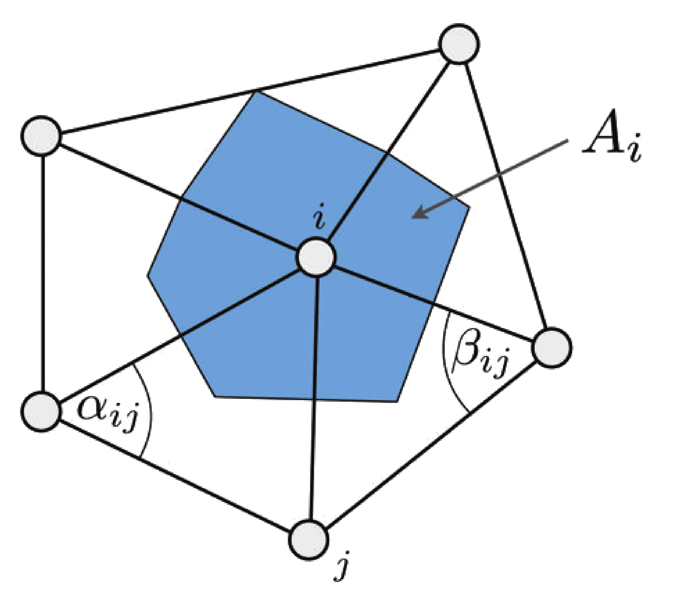
Let's remember the discrete formulation of the Laplace operator over a triangle mesh at a single vertex \( i \):
$$ \Delta f( \vec v_i) = \frac{1} {2A_i} \sum\limits_{{j \in \mathcal N(i)}} { (\cot \alpha_{ij} + \cot \beta_{ij}) (f_j - f_i) } $$
- \( {j \in \mathcal N(i)} \) is the list of vertices directly adjacent to the vertex \( i \)
- \(\cot \alpha_{ij} + \cot \beta_{ij}\) are the infamous cotangent weights (a real value) other type of weights exists but those are the most popular.
- \( f_i, f_j, ...\) the scalar weights at the vertices.
- \( A_i \) is the cell area (a real value). Several solution exists to measure this quantity
Barycentric cell area: Probably the simplest way to compute \( A_i \) just sum the triangles' areas adjacent to \(i\) and take one third:
$$A_i = \frac{1}{3} \sum\limits_{{T_j \in \mathcal N(i)}} {area(T_j)}$$
Mixed Voronoi cell area: more robust, but a bit more painful to compute
float cell_area = 0 // A_i
for( each triangle tri_j from the 1-ring neighborhood of vertex i )
    if( tri_j is non-obtuse) // Voronoi safe
        cell_area += voronoi region of i in tri_j
    else // Voronoi inappropriate
        if( the angle of 'tri_j' at 'i' is obtuse)
            cell_area += area(tri_j)/2.0
        else
            cell_area += area(tri_j)/4.0
The Voronoi region of a triangle with vertex \(\vec p\),\(\vec q\) and \(\vec r\):
$$\frac{1}{8} (\|\vec p - \vec r\|^2 \cot( \text{angle at } \vec q) + \|\vec p - \vec q\|^2 \cot( \text{angle at } \vec r) )$$
Matrix representation (development)
Here things get interesting, we will represent \( \Delta f( \vec v_i) \) at every vertices using matrices so that \( \Delta f = \mathbf A \mathbf x\) with \( \mathbf x = \{ f_0, f_1 \ldots f_i \ldots \} \). We will be able to re-use this matrix in many FEM applications (Finite Element Method), and solve PDEs (Partial Differential Equations) For brevity let's define:
- \( w_{ij} = \frac{1}{2} \cot \alpha_{ij} + \cot \beta_{ij}\)
- \( w_{sum_i} = \sum\limits_{{j \in \mathcal N(i)}} { w_{ij} } \)
We start from the per vertex expression and refactor it:
$$
\begin{array}{lll}
\Delta f( \vec v_i) & = & \frac{1} {A_i} \sum\limits_{{j \in \mathcal N(i)}} { w_{ij} (f_j - f_i) } \\
& = & \frac{1} {A_i} \sum\limits_{{j \in \mathcal N(i)}} { w_{ij} (f_j) } - \frac{1} {A_i}
\left ( \sum\limits_{{j \in \mathcal N(i)}} { w_{ij} } \right ) (f_i) \\
& = & \frac{1} {A_i} \sum\limits_{{j \in \mathcal N(i)}} { w_{ij} (f_j) } - \frac{1} {A_i}
w_{sum_i} (f_i) \\
\end{array}
$$
Now that we properly isolated our \( f_i \) and \( f_j\) (really our \(\mathbf x\)) we can infer the general matrix representation for each vertices (each matrix has the same dimension \( \mathbb R^{n \times n} \).):
$$
\mathbf A \mathbf x =
\overbrace{ {\mathbf M}^{-1} }^{\frac{1} {A_i}} \quad
\overbrace{ \mathbf L_{w_{ij}} \mathbf x }^{ \sum\limits_{{j \in \mathcal N(i)}} w_{ij} f_j }
- {\mathbf M}^{-1}
\overbrace{ \mathbf L_{w_{sum}} \mathbf x }^{ \sum\limits_{{j \in \mathcal N(i)}} w_{ij} f_i }
$$
A example of expansion:
$$
\begin{bmatrix}
A_0 & 0 & 0 \\
0 & A_1 & 0 \\
0 & 0 & A_2\\
\end{bmatrix}^{-1}
\begin{bmatrix}
0 & w_{01} & w_{02} \\
w_{10} & 0 & w_{12} \\
w_{20} & w_{21} & 0 \\
\end{bmatrix}
\begin{bmatrix}
f_0 \\
f_1 \\
f_2 \\
\end{bmatrix}
-
\begin{bmatrix}
A_0 & 0 & 0 \\
0 & A_1 & 0 \\
0 & 0 & A_2\\
\end{bmatrix}^{-1}
\begin{bmatrix}
w_{sum_0} & 0 & 0 \\
0 & w_{sum_1} & 0 \\
0 & 0 &w_{sum_2}\\
\end{bmatrix}
\begin{bmatrix}
f_0 \\
f_1 \\
f_2 \\
\end{bmatrix}
$$
The Mass matrix \( \mathbf M \) is a diagonal matrix that stores the cell area of each vertex; elements outside the diagonal are null:
$$
\mathbf M =
\begin{bmatrix}
A_0 & 0 & 0 \\
0 & \ddots & 0 \\
0 & 0 & A_n\\
\end{bmatrix}
$$
The matrix \( \mathbf L_{w_{sum}} \)
is also a diagonal matrix that stores the sum of the cotangent weights at each vertex \( i \):
$$
\mathbf L_{w_{sum}} =
\begin{bmatrix}
w_{sum_0} & 0 & 0 \\
0 & \ddots & 0 \\
0 & 0 &w_{sum_n}\\
\end{bmatrix}
$$
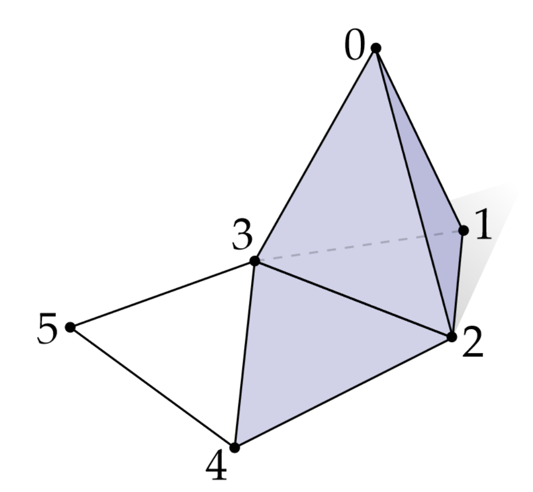
Lastly the Adjacency matrix \( \mathbf L_{w_{ij}} \) is symmetric.
The rows (index \(i\)) and the columns (index \(j\)) represent vertex indices.
If vertex \(\vec v_i\) is directly connected to vertex \(\vec v_j\) then the value of the matrix element \( a_{ij} \) is set to \( w_{ij} \):
$$
\mathbf L_{w_{ij}} =
\begin{bmatrix}
0 & w_{01} & w_{02} & w_{03} & 0 & 0 \\
w_{10} & 0 & w_{12} & w_{13} & 0 & 0 \\
w_{20} & w_{21} & 0 & w_{23} & w_{24} & 0 \\
w_{30} & w_{31} & w_{32} & 0 & w_{34} & w_{35} \\
0 & 0 & w_{42} & w_{43} & 0 & w_{45} \\
0 & 0 & 0 & w_{53} & w_{54} & 0
\end{bmatrix}
$$
The Laplacian matrix definition (digest)
$$
\begin{array}{lll}
\mathbf A \mathbf x & = & {\mathbf M}^{-1} \mathbf L_{w_{ij}} \mathbf x - {\mathbf M}^{-1} \mathbf L_{w_{sum}} \mathbf x \\
& = & ( {\mathbf M}^{-1} \mathbf L_{w_{ij}} - {\mathbf M}^{-1} \mathbf L_{w_{sum}}) \mathbf x \\
& = & {\mathbf M}^{-1} (\mathbf L_{w_{ij}} - \mathbf L_{w_{sum}}) \mathbf x \\
\end{array}
$$
What is commonly called the Laplacian matrix in the literature of geometry processing is:
$$\mathbf L = \mathbf L_{w_{ij}} - \mathbf L_{w_{sum}}$$
$$ \mathbf L_{ij} = \left \{ \begin{matrix} w_{ij} & = & \frac{1}{2} (\cot \alpha_{ij} + \cot \beta_{ij}) & \text{ if j adjacent to i} \\ & ~ & -\sum\limits_{{j \in \mathcal N(i)}} { w_{ij} } & \text{ when } j = i \\ & ~ & 0 &\text{ otherwise } \\ \end{matrix} \right . $$
On the other hand the Laplacian *operator* is defined as:
$$\mathbf {\Delta f} = {\mathbf M}^{-1} \mathbf L$$
A word of caution, be aware that the general Laplacian matrix as defined in graph theory (as opposed to geometry processing) is usually defined as \( -\mathbf L \)
Harmonic weights
To find the values \( \mathbf x = \{ \ldots f_i \ldots \} \) that describe an harmonic function (as linear as possible on x, y z coordinates. We must solve the Laplace equation:
$$
\begin{array}{lll}
& \mathbf {\Delta f} & = & 0 \\
\Rightarrow & {\mathbf M}^{-1} \mathbf L \mathbf x & = & [ 0 ] \\
\Rightarrow & \mathbf L \mathbf x & = & [ 0 ]
\annotation{ \text{Multiply both sides by } \mathbf M}\\
\end{array}
$$
Where \( [ 0 ] \in \mathbb R^n \) is a column vector of zeros.
What is nice with this, is that \( \mathbf L \) is symmetric by construction,
so when we multiply by \( \mathbf M \) to get rid of \( \mathbf M^{-1} \)
we make the linear system of equations simpler.
\( \mathbf L \) is also a sparse matrix,
which means we can take advantage of a sparse solver to find the result of this system even quicker.
Boundary conditions: you need to set a close region such as:
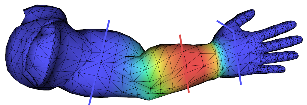
In the above examples we have set the vertices in blue to 0.0, and some vertices of the mid sections in red to 1.0.
Here is how to set a vertex \( i \) to a specific value \(v\). In our linear system \(\mathbf L \mathbf x = [0]\) (a.k.a our linear system of equation \(\mathbf {Ax} = \mathbf{b}\)) set the entire row \( i \) of \(\mathbf L\) to 0 but leave the diagonal element \( \mathbf L_{i,i} = v\). then in the column vector \([0]\) (a.k.a our right hand side \(\mathbf b\)) we set \( b_i = v \). So that we effectively hard set the fact that the ith vertex takes the value \(v\).
Here is an example of such system where we set the value of vertex \(i=2\) to \(v\):
$$ \newcommand{sumw}[1]{ -\sum } \begin{bmatrix} \sumw{0} & w_{01} & w_{02} & w_{03} & 0 & 0 \\ w_{10} & \sumw{1} & w_{12} & w_{13} & 0 & 0 \\ 0 & 0 & 1 & 0 & 0 & 0 \\ w_{30} & w_{31} & w_{32} & \sumw{3} & w_{34} & w_{35} \\ 0 & 0 & w_{42} & w_{43} & \sumw{4} & w_{45} \\ 0 & 0 & 0 & w_{53} & w_{54} & \sumw{5} \end{bmatrix} \begin{bmatrix} x_0 \\ x_1 \\ x_2 \\ x_3 \\ x_4 \\ x_5 \\ \end{bmatrix} = \begin{bmatrix} 0 \\ 0 \\ v \\ 0 \\ 0 \\ 0 \\ \end{bmatrix} $$Note: go here to find harmonic weights on a regularly spaced grid.
C++ Code
I provide [ ![]() code ] to solve the laplace equation with Eigen results are displayed with free GLUT. In
code ] to solve the laplace equation with Eigen results are displayed with free GLUT. In solve_laplace_equation.cpp you will find code similar to the snippet below, that builds the Laplacian matrix with cotan weights set the boundary conditions by zeroing out rows of the final matrix setting its diagonal element to 1 and right hand side of the equation to the desired value.
If your mesh is represented with an half-edge data structure (each vertex knows its direct neighboors) the pseudo code to compute \( \mathbf L \) is:
 // angle(i,j,t) -> angle at the vertex opposite to the edge (i,j)
for(int i : vertices) {
    for(int j : one_ring(i)) {
        sum = 0;
        for(int t : triangle_on_edge(i,j))
        {
            w = cot(angle(i,j,t));
            L(i,j) = w;
            sum += w;
        }
        L(i,i) = -sum;
    }
}
On the other hand the Laplacian \( \mathbf L \) may be built by summing together contributions for each triangle, this way only the list of triangles is needed:
for(triangle t : triangles)
{
    for(edge i,j : t)
    {
        w = cot(angle(i,j,t));
        L(i,j) += w;
        L(j,i) += w;
        L(i,i) -= w;
        L(j,j) -= w;
    }
}
References
- Book: Geometry Mesh Processing, Mario Botsch & al
- Discrete Differential-Geometry Operators for Triangulated 2-Manifolds Meyer & al
- Laplace-Beltrami: The Swiss Army Knife of Geometry Processing
 Donate
No comments