2D biharmonic stencil a.k.a bilaplacian operator

Draft / notes / memo

The Bi-harmonic stencil can be inferred from the harmonic stencil. By applying the harmonic stencil to itself with the convolution operator we obtain the biharmonic stencil.

Recall that the harmonic stencil (a.k.a the Laplace operator) is:

\[ \Delta f(x,y) \approx \frac{f(x-h,y) + f(x+h,y) + f(x,y-h) + f(x,y+h) - 4f(x,y)}{h^2}, \]

    1
 
1  -4   1

    1

Note: finding the harmonic stencil can be simply done by summing the 2nd derivative central finite difference (first order accuracy)
Advanced example of application of the harmonic stencil to solve a PDE

So the biharmonic stencil is represented figure 2.2 below:

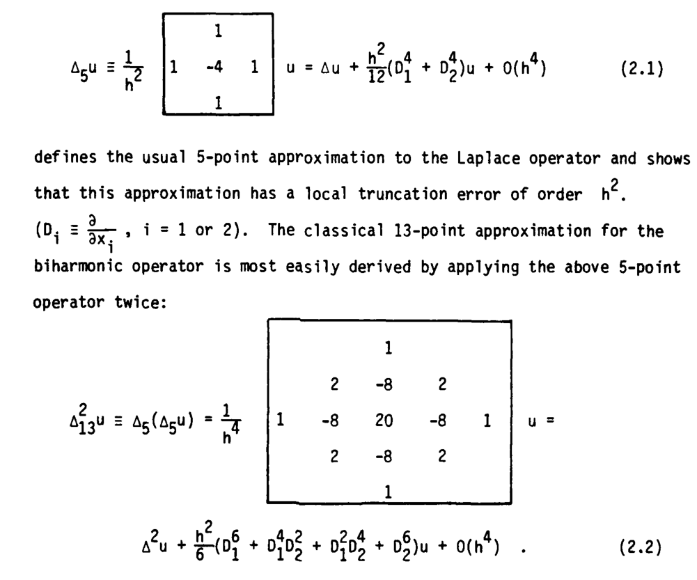
The above image is from: harmonic and biharmonic stencil (local host) or here

For biharmonic weights on triangle mesh look at my other article

To look into as well: FinDiff is a python package that computes finite difference stencils and coefficients in any dimension, and can numerically compute derivatives or solve PDEs.

Localized bi-Laplacian Solver on a Triangle Mesh and Its Applications alt link

1d biharmonic stencil is (see https://en.wikipedia.org/wiki/Finite_difference_coefficient):

(1 -4 6 -4 1)

which you can infer by applying the harmonic stencil (1 -2 1) to itself.

Here we apply the biharmonic stencil iteratively, it should converge to biharmonic weights.

template< typename T>
void diffuse_biharmonic(Grid2_ref grid,
                        Grid2_const_ref mask,
                        int nb_iter = 128*16)
{
    tbx_assert( grid.size() == mask.size());
    Vec2_i neighs_1[4] = {Vec2_i( 1, 0),
                         Vec2_i( 0, 1),
                         Vec2_i(-1, 0),
                         Vec2_i( 0,-1)};

    Vec2_i neighs_2[4] = {Vec2_i( -1, -1),
                         Vec2_i( -1,  1),
                         Vec2_i(  1,  1),
                         Vec2_i(  1, -1)};

    // First we store every grid elements that need to be diffused according
    // to 'mask'
    int mask_nb_elts = mask.size().product();
    std::vector idx_list;
    idx_list.reserve( mask_nb_elts );
    for(Idx2 idx(mask.size(), 0); idx.is_in(); ++idx) {
        if( mask( idx ) == 1 )
            idx_list.push_back( idx.to_linear() );
    }

    // Diffuse values with a Gauss-seidel like scheme
    for(int j = 0; j < nb_iter; ++j)
    {
        // Look up grid elements to be diffused
        for(unsigned i = 0; i < idx_list.size(); ++i)
        {
            Idx2 idx(grid.size(), idx_list[i]);

            T sum  = T(0);
            T mean = T(0);

            for(int i = 0; i < 4; ++i)
            {
                Idx2 idx_neigh = idx + neighs_1[i];
                if( idx_neigh.is_in() /*check if inside grid*/ ){
                    T weight = (T)8;
                    sum = sum + grid( idx_neigh ) * weight;
                    mean += weight;
                }
            }

            for(int i = 0; i < 4; ++i)
            {
                Idx2 idx_neigh = idx + neighs_2[i];
                if( idx_neigh.is_in() /*check if inside grid*/ ){
                    T weight = (T)-2;
                    sum = sum + grid( idx_neigh ) * weight;
                    mean += weight;
                }
            }

            for(int i = 0; i < 4; ++i)
            {
                Idx2 idx_neigh = idx + neighs_1[i] * 2;
                if( idx_neigh.is_in() /*check if inside grid*/ ){
                    T weight = (T)-1;
                    sum = sum + grid( idx_neigh ) * weight;
                    mean += weight;
                }
            }

            sum = sum / (T)( mean );
            grid( idx ) = sum;
        }
    }
}

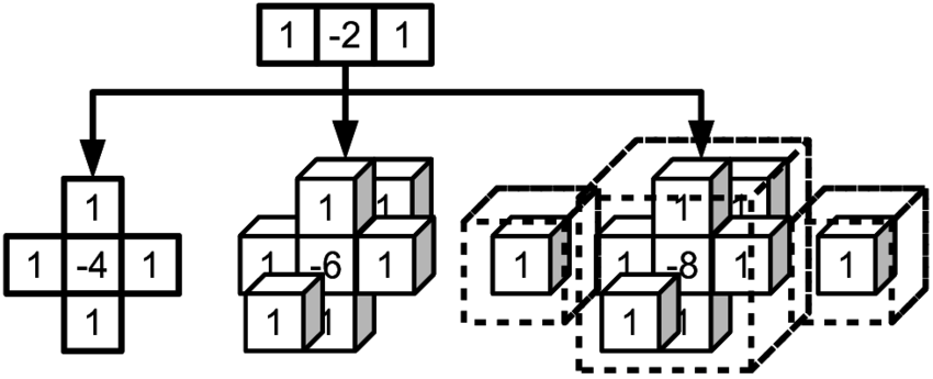
Related: 3D laplacian Just a comment: In Finite Differences, it can be much convenient to write it in terms of Kronecker products: if $A$ is the classical $[1,-2,1]$ matrix, you have that the 3D Laplacian is $$A = I \otimes I \otimes A + I \otimes A \otimes I + A \otimes I \otimes I$$ where $I$ is the identity matrix.

Paper to check out: Automated and Parallel Code Generation for Finite-Differencing Stencils with Arbitrary Data Types which describes the 2d and 3d laplacian and bilaplacian.

Note: Biharmonic functions minimize Laplacian energy

Other related stuff

Biharmonic distance (based on cotan weights)

Biharmonic Coordinates

One comment

Name

Email (optional field, I won't disclose or spam but it's necessary to notify you if I respond to your comment)

All html tags except <b> and <i> will be removed from your comment. You can make links by just typing the url or mail-address.

Anti-spam question:
√4 + 40 = ?

Day of inquiry. You will be subpoenaed.