Curvature of a triangle mesh, definition and computation.

How to compute the curvature for a triangular 3d mesh - 05/2013 - #Geometry

Defining and giving the formula to compute the curvature over a triangle mesh at some vertices.

Normal curvature

By intersecting a surface with a plane we see that the section defines a curve:

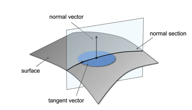
The curvature of this curve is called 'normal curvature' and noted $ k_n$ because the plane is spanned through the normal $ \boldsymbol n$ and an arbitrary tangent vector $ \boldsymbol t $. Now, given a point $ \boldsymbol p $ on the surface you can find an infinity of curvatures given the direction you choose for your tangent vector $ \boldsymbol t $.

Principal curvatures

But how can we characterize the curvature of a surface at a given point when we seem to have an infinity of curvatures? Don't worry! It can be shown that when rotating the normal plane around $ \boldsymbol n $ you can always find two 'principal curvatures' $ k_1 $ and $ k_2 $ respectively defining the maximal and minimal curvature at a given point $ \boldsymbol p $ of the surface:

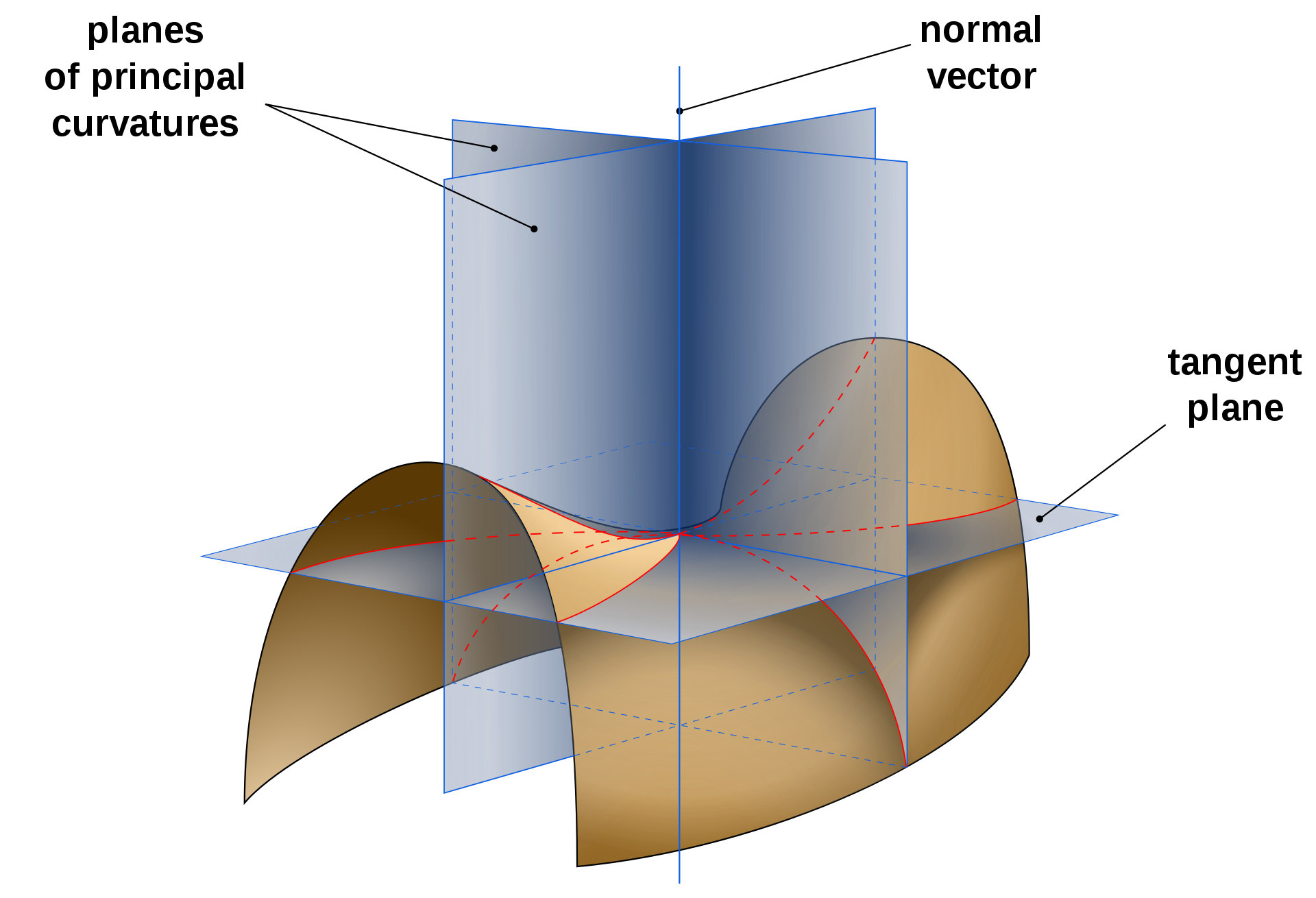
In addition, the principal curvatures $ k_1 $ and $ k_2 $ are associated to the 'principal directions' $ \boldsymbol t_1 $ and $ \boldsymbol t_2 $ which are always found to be orthogonal to each other! What's more, you can define any 'normal curvature' $ k_n $ as a combination of the principal curvatures $ k_1 $ and $ k_2 $ using Euler's theorem below:

\[ k_n = k_1\cos^2\theta + k_2\sin^2\theta \]

Where $ \theta $ is the angle between $ \boldsymbol t_1 $ (maximal curvature direction) and $ \boldsymbol t_n $ the normal curvature.

Calculation

One can compute the principal curvatures $ k_1 $ and $ k_2 $ according to the Mean curvature $ H $ and the Gaussian curvature $ k_g $, don't worry we will define both $ H $ and $ k_g $ in the next sections:

$$ \begin{align*} k_1 & = H + \sqrt{ H^2 - k_g} \\ k_2 & = H - \sqrt{ H^2 - k_g} \end{align*} $$

Gaussian curvature

The Gaussian is the product of principal curvatures $k_1$ and $k_2$:

\[ k_g = k_1 * k_2 \]

on a triangular mesh it can be computed at vertex $ \boldsymbol p_i $ as follows:

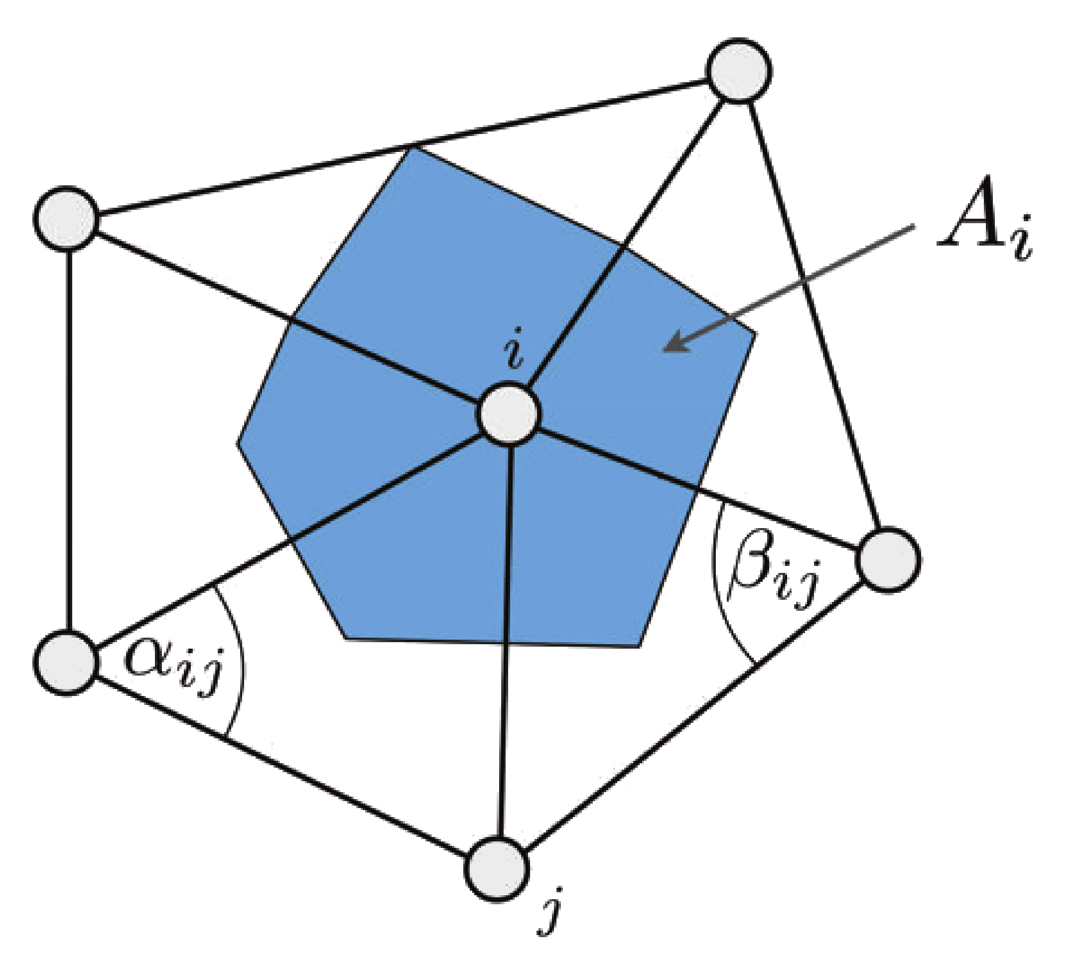
\[ k_g = \frac{ 2 \pi - \sum \theta_j } { A_i } \]

Where the angle $ \theta_j $ is defined as:

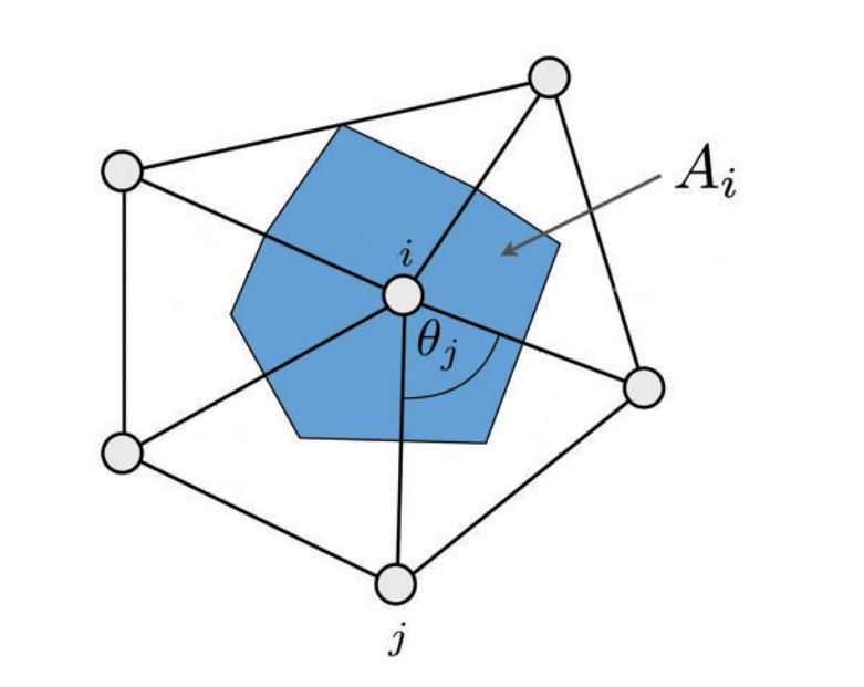
$ A_i $ can be computed as:

'mixed voronoi area'.
'barycentric cell area' (One third of the sum of the triangles' area adjacent to $i$): $ A_i = \frac{1}{3} {\sum\limits_{{T_j \in \mathcal N(i)}} {area(T_j)}} $

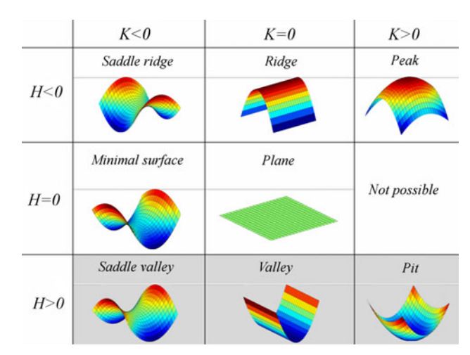
Interpreting the Gaussian curvature's value

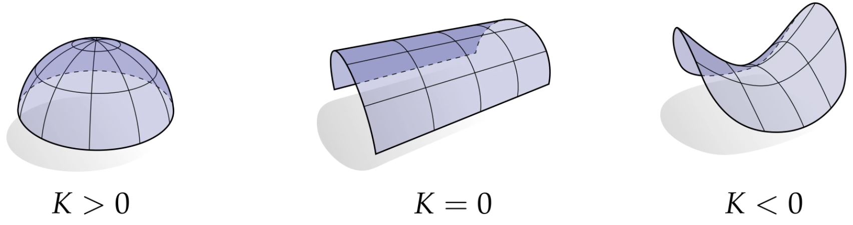
It can help to locally characterize the shape:

$ k_g > 0$ means surface is locally a bowl-like shape. (elliptical point)
$ k_g = 0$ means surface is locally flat in at least one direction (parabolic point)
$ k_g < 0$ means surface is locally a saddle-like shape. (hyperbolic point)

Mean curvature

The mean curvature is the average of the principal curvatures:

$$ H= \frac { k_1 + k_2 } { 2 } $$

In the smooth setting the mean curvature is the average of the normal curvatures in $[0 - 2\pi]$

$$ \begin{align*} k_h & = \frac{1}{2\pi} \int_0^{2\pi} { k_n(\theta) \, d\theta } \\ & \text{ recall the relationship between principal and normal curvature:} \\ k_h & = \frac{1}{2\pi} \int_0^{2\pi} { k_1\cos^2(\theta) + k_2\sin^2(\theta) \, d\theta } \\ \end{align*} $$

If you're lazy like me you can solve this with Maxima , just insert in Maxima's command line:

    ratsimp(1/(2*%pi)*integrate(k1*cos(t)^2 + k2*sin(t)^2, t, 0, 2*%pi));

step by step development:

$$ \newcommand{annotation}[1]{ ~~~~~~\raise 0.8em {\color{grey}\scriptsize{ #1 }} } \begin{align*} k_h & = \frac{1}{2\pi} \left[ \int_0^{2\pi} { k_1 \cos^2(\theta) \, d\theta } \, {\color{red}+} \int_0^{2\pi} {k_2\sin^2(\theta) \, d\theta } \right] \annotation{ \int a + b = \int a + \int b } \\ k_h & = \frac{1}{2\pi} \left[ {\color{red}k_1} \int_0^{2\pi} { \cos^2(\theta) \, d\theta } + {\color{red}k_2} \int_0^{2\pi} {\sin^2(\theta) \, d\theta }\right] \annotation{ \int a.f(x) = a.\int f(x) } \\ k_h & = \frac{1}{2\pi} \left[ k_1\int_0^{2\pi} { {\color{red}\frac{1+ \cos(2\theta)}{2}} \, d\theta } + k_2 \int_0^{2\pi} {{\color{red}\frac{1 - \cos(2\theta)}{2}} \, d\theta }\right] \annotation{ \href{https://en.wikipedia.org/wiki/List_of_trigonometric_identities#Power-reduction_formulae}{\text{Power reduction formulae}} } \\ k_h & = \frac{1}{{\color{red}4}\pi} \left[ k_1 \int_0^{2\pi} { {1+ \cos(2\theta)} \, d\theta } + k_2 \int_0^{2\pi} {{1 - \cos(2\theta)} \, d\theta } \right]\\ k_h & = \frac{1}{4\pi} \left[ k_1 \int_0^{2\pi} {1\, d\theta} \, {\color{red}+} k_1 \int_0^{2\pi}{ \cos(2\theta) \, d\theta } + k_2 \int_0^{2\pi} {1\, d\theta} \,{\color{red}-} k_2 \int_0^{2\pi}{ \cos(2\theta) \, d\theta }\right] \\ k_h & = \frac{1}{4\pi} \left[ k_1 {\color{red} \left [ x \right ]_{0}^{2\pi}} + k_1 \int_0^{2\pi}{ \cos(2\theta) \, d\theta } + \cdots \right] \annotation{ \frac{d(x + c)}{dx} = 1 } \\ k_h & = \frac{1}{4\pi} \left[ k_1 {\color{red} \left [ 2\pi - 0 \right ]} + k_1 {\color{red} \left [ \frac{\sin(2\theta)}{2} \right ]_{0}^{2\pi}} + \cdots \right] \annotation{ \text{chain rule:} f'(g(x)) = g'(x)f'(g(x)) \text{ so, } \frac{d}{dx} ( \frac{1}{2} \, \sin(2x) + c ) = \frac{2}{2} \, \cos(2x) } \\ k_h & = \frac{1}{4\pi} \left[ k_1 {\color{red} 2\pi} + k_1 {\color{red} \left [ \frac{\sin(4\pi)}{2} - \frac{\sin(0)}{2} \right]} + \cdots \right]\\ k_h & = \frac{1}{4\pi} \left[ k_1 2\pi + k_1 {\color{red} 0} + \cdots \right] ~~~~~~\raise 0.8em {\color{grey}\scriptsize{ sin(0) = sin(2\pi) = sin(4\pi) = 0 }} \\ k_h & = \frac{1}{4\pi} \left[ k_1 2\pi + k_2 {\color{red} 2\pi } - k_2 {\color{red} 0} \right]\\ k_h & = \frac{1}{2} \left[ k_1 + k_2 \right] \\ \end{align*} $$ 🥲

In addition, the mean-curvature can also be expressed using the Laplace operator. Below is the mean-curvature normal which norm corresponds to the amount of curvature $ H $:

$$ \frac{\Delta p_i}{2} = -Hn $$

We designate the norm as the absolute mean-curvature:

$$ |H| = \frac{ \| \Delta p_i \|}{ 2 } $$

Mean-curvature sign: the sign of the dot product between the normal of a mesh $\vec n$ and the mean-curvature normal $dot(\vec n_i, -\Delta p_i) $ gives the sign of the mean-curvature $H$. (One can compute $\vec n$ averaging face's normals around a vertex for instance.) This is why we say the mean-curvature is an "extrinsic" property, since the sign of $H$ depends on the orientation of the normal of the mesh.

In other words, to find the mean-curvature normal of a triangle mesh, we need to apply the discrete Laplace operator at some vertex $ \boldsymbol p_i $ as follows:

$$ \Delta \vec p_i = \frac{1} {2A_i} \sum\limits_{{j \in \mathcal N(i)}} { (\cot \alpha_{ij} + \cot \beta_{ij}) (p_j - p_i) } $$

$ {j \in \mathcal N(i)} $ is the list of vertices directly adjacent to the vertex $ i $
$\cot \alpha_{ij} + \cot \beta_{ij}$ are the famous cotangent weights (a real value)
$ p_i, p_j, ...$ vertices position.
$ A_i $ is the cell area as described earlier (a real value).

Note: Alternate discretization of the Laplacian operator could be used. For instance, a rather crude option is to set $(\cot \alpha_{ij} + \cot \beta_{ij}) = 1$. In other words, we simply compute the barycenter of our mesh cell. Although simpler to implement, we lose a great deal of accuracy this way:

$$ \Delta \vec p_i = \frac{1} { |\mathcal N(i)| } \sum\limits_{{j \in \mathcal N(i)}} { 1 . (p_j - p_i) } \\ = \left ( \frac{1} { |\mathcal N(i)| } \sum\limits_{{j \in \mathcal N(i)}} { p_j } \right ) - p_i $$

$|N(i)|$ : number of adjacent vertices to $i$.

Interpreting the Mean curvature's value

$H$ gives the amount of curvature in one way or another as well as the orientation when applicable:

$ H = 0 $ -> saddle or flat surface
$ H < 0 $ -> amount of convexity (peak)
$ H > 0 $ -> amount of concavity (pit)

Smoothing

Interestingly the mean-curvature normal is related to mesh smoothing algorithm, since smoothing (sometimes designated as curvature flow) can be seen as minimizing the mean-curvature.

Gaussian VS Mean curvature

Notice how $ H < 0 $ or $ H > 0 $ virtually describes the same shape, the difference between a peak and a pit is a matter of perspective. Ultimately it is set according to the convention you use to define the mean-curvature's sign.

Code

Gaussian curvature in libigl
Mean-curvature in libigl

Code sample explained:

// a list of 3d vectors that represents the mean-curvature normals (H x n)
MatrixXd HN; // size: nb_verts x 3
SparseMatrix<double> L; // Laplacian matrix (nb_verts x nb_verts)
SparseMatrix<double> M; // Mass matrix (diagonal matrix where each diagonal element a_i == the cell area at the ith vertex)
SparseMatrix<double> Minv; // inverse of the mass matrix (so 1.f/a_i)
igl::cotmatrix(V,F,L); // computes L, the variables V and F are just the list of Vertex and triangle Face index
igl::massmatrix(V,F,igl::MASSMATRIX_TYPE_VORONOI,M); // Compute M
igl::invert_diag(M,Minv); // Compute the inverse of M
HN = -Minv*(L*V); // Minv*L => is the Laplace operator, multiplying Minv*L against the list of vertices V is equivalent to applying the operator (\Delta p)
H = HN.rowwise().norm(); //up to sign <- absolute mean-curvature

More accurate approaches to compute mean curvature also includes:

- Approach based on dihedral angles
- Quadric fitting

JavaScript

JavaScript library to compute Gauss/Mean and principal curvatures. The corresponding online demo is here. Find more information at the main project page.

Other hacks

When accuracy is not an issue, for instance you just roughly want to detect pits and darken them or colorize them for artistic purpose, there are other more hacky/simpler ways to compute curvature:
- https://blender.stackexchange.com/a/147371/126011
- https://computergraphics.stackexchange.com/a/1719/16151

References

- Discrete Differential-Geometry Operators for Triangulated 2-Manifolds Mark Meye & Al
- Polygon mesh processing by Mario Bosch & Al
- Discrete Differential Operators for Computer Graphics (Mark Meyer's thesis)
- Alec Jacobson geometry processing course: "discrete-mean-curvature-normal-via-discrete-laplace"

Donate

two comments

The ‘barycentric cell area’ is not “sum of the triangles’ area adjacent to i times 3”, but “sum of the triangles’ area adjacent to i divided by 3”

From page 10 in [http://www.geometry.caltech.edu/pubs/DMSB_III.pdf]:
“It is interesting to notice that using the barycentric area as an averaging
region results in an operator very similar to the definition of the mean cur-
vature normal by Desbrun et al. [DMSB99], since A_Barycenter is a third of the
whole 1-ring area A_1-ring used in their derivation.”
——————————
Rodolphe: Nice catch, thank you!

Felix - 10/10/2022 -- 21:51

Hello, there seems to be a mismatch between “Interpreting the Mean curvature’s value” and the figure in the following section:

text: H > 0 -> peak, image: H < 0 -> pit
text: H < 0 -> pit, image: H < 0 -> peak

I think the sign depends on the convention you use, however, it should be consistent.
——————-
Rodolphe: Thank you for helping improve this article! 🙏

Best regards!

Victor - 29/05/2024 -- 10:48

Rodolphe Vaillant's homepage

Research, teaching and more...